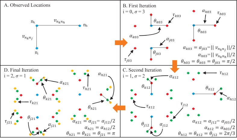
Figure 1.

A step-by-step visual representation of the algorithm in Box 1 on a network of K = 3 observed discrete sampling locations with τ = 3. A) The three observed sampling locations (n_h, n_j, n_k) are shown as blue circles and the corresponding shortest vectors are $v_{n_k{n}_j}$ and $v_{n_k{n}_h}$. B) Each observed location is given σ = 3 nodes (τ_h03, τ_j03, τ_k03) shown as red circles. These nodes are distributed by (3) and (4). C) Each red node is given σ = 2 nodes (τ_h12, τ_j12, τ_k12) shown as green circles, distributed by (3) and (5). D) Each green circle is given σ = 1 node, (τ _h21, τ_j21, τ_k21) shown as yellow circles, distributed by (3) and (5). At this point there are no new nodes to add and the algorithm exits. There are ϕ(3, 3) = 48 total nodes in the new set by (6) and (7). The distances and angles between nodes are shown by α_xyz and θ_xyz, respectively, where x is the node (h, j, k), y is the i^th step in the iteration, and z is the count of σ nodes added during the step. Note that all α and θ values are equal for each node for each step in the algorithm.