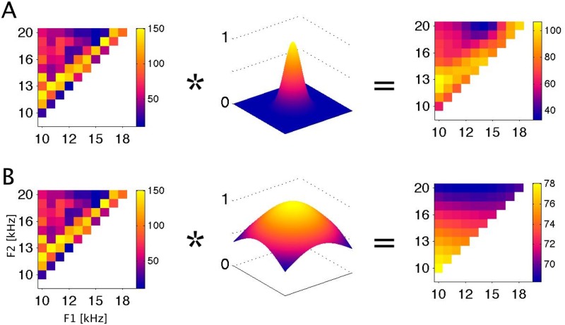
Fig 4. Smoothing of an FRF with 2-dimensional Gaussian smoothing filters.
A: smoothing with a 0.1 octave wide filter. B: smoothing with a 0.5 octave wide filter. Left panels: The original FRF is same example as the one in Fig 3E. FRFs are plotted as in Figs 2 and 3, with formant frequencies in kHz on the coordinate axes, and the color scale giving spike rates in Hz. Middle panels: 2-dimensional Gaussian filters with σ = 0.1 (A) or σ = 0.5 (B) octaves standard deviation. Right panels: The result of convolving the FRF with the smoothing filter. To determine the ‘best’ σ for individual FRFs we use a cross-validation method described in Fig 5.

