Extended Data Figure 1. Decomposition-based peak identification (DPI).

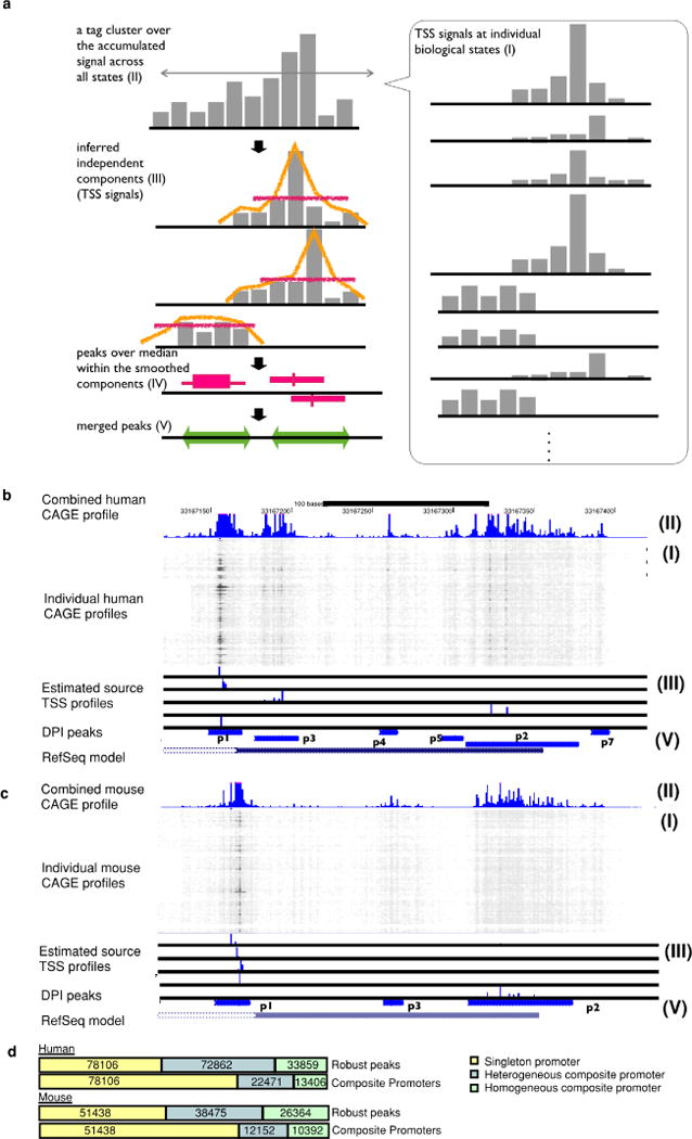
a, Schematic representation of each step in the peak identification. This starts from CAGE profiles at individual biological states (I), subsequently defines tag clusters (consecutive genomic region producing CAGE signals) over the accumulated CAGE profiles across all the states (II). Within each of the tag cluster, it infers up to five underlying signals (independent components) by using ICA independent component analysis (ICA) (III). It smoothens each of the independent components and finds peaks where signal is higher than the median (IV). The peaks along the individual components are finally merged if they are overlapping each other (V). b, c, Genomic view of actual examples (B4GALT1 locus) for human and mouse. CAGE profiles across the biological states (I) are shown as a greyscale plot, in which the x axis represents the genomic coordinates and individual rows represent individual biological states. Dark (or black) dots indicate frequent observation of transcription initiation (that is, larger number of CAGE read counts) and light dots (white) indicate less frequency. The blue histogram on the top indicates the accumulated CAGE read counts, and the entire region shown represents a single tag cluster (II). The histograms below the greyscale plot indicate the independent components of the CAGE signals inferred by ICA (III), and the resulting CAGE peaks are shown at the blue bars closest to the bottom (V). The bottom track indicates a gene model in RefSeq. The figures overall indicate that only one TSS is defined by RefSeq gene models in this locus, however, transcription starts from slightly different regions depending on the context, and the DPI method successfully captured the different initiation events. d, Breakdown of singleton and composite transcription initiation regions with homogenous or heterogeneous expression patterns according to likelihood ratio test (see Supplementary Methods).