FIG. 6.

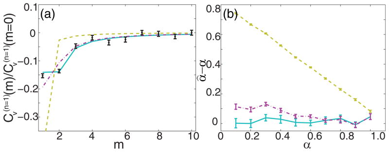
(Color online) Illustrative example of n = 1 VAC analysis of 2D simulated data for D^* = 0.01μm²/s^α, t_E = 10 ms, p̄ = 1000, and b = 0. The ensemble consisted of 100 tracks of length 100 frames each. Offsets due to static error have been removed by first estimating σ₀ for the specified photon statistics. Error bars reflect the S.E.M. from 100 bootstrapped samples of the ensemble. In both panels the gold dashed line corresponds to the VAC without inclusion of dynamic error, the magenta dashed-dotted line corresponds to the intermediate treatment of dynamic error as described in the text, and the cyan solid line corresponds to the full treatment of dynamic error. (a) Example computed VAC for α = 0.2 (black dots and error bars) and the corresponding predicted curves for each treatment of dynamic error. The point at m = 1 is not plotted for the sake of scaling the figure and since each scaled VAC is equal to 1 here by definition. (b) Bias in the estimate of α for various α.