Assessing Effects of Prenatal Alcohol Exposure Using Group-wise Sparse Representation of FMRI Data

Abstract

Task-based fMRI activation mapping has been widely used in clinical neuroscience in order to assess different functional activity patterns in conditions such as prenatal alcohol exposure (PAE) affected brains and healthy controls. In this paper, we propose a novel, alternative approach of group-wise sparse representation of the fMRI data of multiple groups of subjects (healthy control, exposed non-dysmorphic PAE and exposed dysmorphic PAE) and assess the systematic functional activity differences among these three populations. Specifically, a common time series signal dictionary is learned from the aggregated fMRI signals of all three groups of subjects, and then the weight coefficient matrices (named statistical coefficient map (SCM)) associated with each common dictionary were statistically assessed for each group separately. Through inter-group comparisons based on the correspondence established by the common dictionary, our experimental results have demonstrated that the group-wise sparse coding strategy and the SCM can effectively reveal a collection of brain networks/regions that were affected by different levels of severity of PAE.

1. INTRODUCTION

Task-based fMRI has been widely used to identify brain regions that are functionally involved in specific task performance, and has significantly advanced our understanding of functional localizations within the brain (Friston et al., 1994; Heeger and Ress, 2002; Matthews and Jezzard, 2004; Logothetis et al., 2008). In the functional neuroimaging community, there have been a variety of model-based or data-driven approaches for fMRI time series analysis and/or activation detection, for instances, correlation analysis (Bandettini et al., 1993), general linear model (GLM) (Friston et al., 1994; Worsley, 1997), statistic testing (Ardekani et al., 1998), principal component analysis (PCA) (Andersen et al., 1999), Markov random field (MRF) models (Descombes et al., 1998), mixture models (Hartvig and Jensen, 2000), independent component analysis (ICA) (McKeown et al., 1998), clustering analysis (Baumgartner et al., 1997), wavelet algorithms (Bullmore et al., 2003; Shimizu et al., 2004), autoregressive spatial models (Woolrich et al., 2004a), Bayesian approaches (Huaien and Puthusserypady, 2007; Bowman et al., 2008), and empirical mean curve decomposition (Deng et al., 2012). Among all of these methods, GLM is one of the most widely used methods (Friston et al., 1994; Worsley et al., 1997) due to its effectiveness, simplicity and robustness. In particular, several popular fMRI data analysis software packages such as the FSL FEAT (http://www.fmrib.ox.ac.uk/fsl/feat5/index.html), SPM (http://www.fil.ion.ucl.ac.uk/spm/) and AFNI (http://afni.nimh.nih.gov/afni/) have employed the GLM method (Friston et al., 1994; Worsley et al., 1997).

In addition to the abovementioned voxel-wise methods, in order to deal with the remarkable individual variability and different sources of noises (e.g., Thirion et al., 2007; Derrfuss and Mar, 2009; Laird et al., 2009; Hamilton, 2009; Costafreda, 2009; Tahmasebi, 2010), group-wise task fMRI activation detection methods have been developed, such as the two-level group-wise GLM method (Beckmann et al., 2003), Bayesian inference (Woolrich et al., 2004b), multi-level analysis (Thirion et al., 2007), group ICA analysis (Calhoun et al., 2009), FENICA (Schöpf et al.,2011), group Markov Random Field (MRF) methods (Ng et al., 2010), and our recently developed DICCCOL-based group-wise activation detection (Lv et al., 2014a). For instance, the FSL FEAT/FLAME toolkits (Beckmann et al., 2003; Smith et al., 2004) incorporated a two-level group-wise GLM analysis procedure that warps the individual activation significance maps to the same template space via image registration methods (e.g., FSL FLIRT), and then infers the group-wise significantly activated regions from the pooled activation maps. The major advantages of this two-level GLM method include the facilitation of valid group analyses and inference, good flexibility and generality, and easy and meaningful interpretation of results (Beckmann et al., 2003; Smith et al., 2004). In our recently developed DICCCOL (dense individual and common connectivity-based cortical landmarks)-based group-wise activation detection (Lv et al., 2014a), the first-level GLM analysis was first performed on the fMRI signal of each corresponding DICCCOL landmark in individual brain’s own space, and then the estimated effect sizes of the same landmark from a group of subjects are statistically assessed with the mixed-effect model at the group level. Finally, the consistently activated DICCCOL landmarks are determined and declared in a group-wise fashion in response to external block-based stimuli. The advantage of this method is that these statistical inferences based on the intrinsically-established DICCCOL correspondences among a group of subjects can be more reliable and robust to the variability in individual activation magnitudes and the evoked brain networks.

Although these abovementioned methods leveraged the statistical power from multiple brains in order to gain the robustness to noises and the less sensitivity to individual variability, challenges still exist. First, although the statistical activation maps can be estimated group-wisely in spite of the variability of individual anatomy with image registration methods, the consistency and diversity of dynamic temporal responses evoked by task performance cannot be systematically assessed group-wisely. Second, it has been difficult to model multiple concurrent brain responses from different spatially-overlapping brain networks. Specifically, from a human neuroscience perspective, it has been widely reported and argued that a variety of cortical regions and networks exhibit strong functional diversity (Duncan, 2010; Gazzaugia, 2004; Pessoa, 2012), that is, a cortical region could participate in multiple functional domains/processes and a functional network might recruit various heterogeneous neuroanatomic areas (Gazzaugia, 2004; Pessoa, 2012). Therefore, it is possible that heterogeneous regions and diverse activities participating in a task performance could be overlooked by brain activity modeling methods. As a consequence, it is challenging for model-driven task fMRI data analysis methods to reconstruct concurrent functional networks and assess systematic activity differences across populations.

In recognition of the above challenges, researchers, including ourselves, have decomposed fMRI signals into linear combinations of multiple components based on data-driven sparse representation of whole-brain fMRI signals (Lee et al., 2011; Lv et al., 2013; Lv et al., 2014b; Lv et al., 2015; Varoquaux et al., 2011). The basic idea of this computational methodology is to aggregate all of dozens (or hundreds) of thousands of fMRI signals within the whole brain of one subject into a big data matrix, which is subsequently factorized into an over-complete dictionary basis matrix and a reference weight matrix via dictionary learning and sparse coding algorithms (Mairal et al., 2010). Then, the time series of each over-complete basis dictionary represents the functional activities of a brain network and its corresponding reference weight vector stands for the spatial map of this brain network (Lv et al., 2013; Lv et al., 2014b; Lv et al., 2015). An important characteristic of this framework is that the decomposed reference weight matrix naturally reveals the spatial overlap/interaction patterns among reconstructed brain networks (Lv et al., 2014b). Thus this novel data-driven strategy naturally accounts for that a brain region might be involved in multiple functional processes (Duncan, 2010; Gazzaugia, 2004; Pessoa, 2012) and its fMRI signal is composed of various components (Lee et al., 2011; Lv et al., 2013; Lv et al., 2014b; Lv et al., 2015; Varoquaux et al., 2011).

However, an unsolved problem in previous methods of sparse representation of fMRI signals (Lee et al., 2011; Lv et al., 2013; Lv et al., 2014b; Varoquaux et al., 2011) is how to establish the correspondence of different dictionary components across individuals and populations. Specifically, works in (Lee et al., 2011; Lv et al., 2014b; Lv et al., 2015) performed dictionary learning and sparse coding on whole brain fMRI signals and interesting functional networks of meaningful temporal and spatial patterns can be detected among all the learned components. But it is difficult to perform inter-subject comparison or statistical analysis mainly because the data-driven dictionary learning and sparse coding method applied on individuals learned brain networks by taking account of individual specificity adaptively (Lee et al., 2011; Lv et al., 2014b), and correspondence cannot be established across subjects. A common dictionary is learned from the task fMRI signals of a group of subjects in Lv et al., 2013, so that group-wise analysis could be established based on the correspondence of the common dictionary basis. However, inter-group comparison is usually required for clinical research such as assessing the differences of functional brain activities between brain conditions such as prenatal alcohol exposure (PAE) (Coles et al., 1991; Santhanam et al. 2009) and healthy controls. So far, establishing correspondence across groups as well as across subjects is an important problem that has not been sufficiently investigated before. Another important issue is the variability in fMRI analysis and group-wise methods. In other words, there is remarkable variability of activation magnitudes for the corresponding brain regions across individual subjects and imaging sessions (Smith et al., 2005; Thirion et al., 2007), due to physiological noises, head/body motion, resting-state activity and other factors. This variability imposes additional challenges to the robust and reliable inference of group-wise consistent functional networks.

In responses to the above challenges, in this paper, we propose a novel computational framework of group-wise sparse representation of the fMRI datasets of multiple groups of subjects (healthy control, exposed non-dysmorphic PAE and exposed dysmorphic PAE (Santhanam et al., 2009) and comprehensively assess the systematic functional activity differences among these three populations. Specifically, fMRI signals from all of the three groups of subjects are aggregated as training samples to learn a common time series signal dictionary, which would establish component correspondence across subjects and groups. Before the extraction of fMRI signals, each subject has been registered into the MNI atlas space, in which the voxel correspondence is roughly established across all subjects and groups based on a unified brain mask which covers common region of all brains. After sparse coding using the online dictionary method (Mairal et al., 2010), statistical assessment is performed on the weight coefficient matrices, named statistical coefficient map (SCM) here, associated with each common dictionary for each group separately. By comparing the inter-group differences based on the correspondence established by the common dictionary, our experimental results demonstrated that the group-wise sparse coding strategy can effectively elucidate different levels of effect of PAE in a collection of brain networks/regions.

2. MATERIALS AND METHODS

2.1. Overview

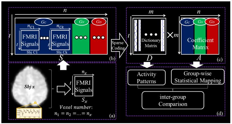
Our computational pipeline is summarized in Fig.1. First, subjects from 3 groups (GC: Healthy control, GN: Non-dysmorphic PAE, GD: Dysmorphic PAE (Santhanam et al., 2009) are spatially normalized into the standard MNI space via linear image registration method FSL FLIRT (Jenkinson et al., 2001). Then, by using a standardized group common brain mask, whole-brain fMRI signals of each subject are extracted and aggregated into a 2D signal matrix S_x ∈ ℝ^t×n_x, as shown in Fig.1a. Then all extracted signal matrices from 3 groups are pooled and arranged into a big matrix S∈ ℝ^t×n as shown in Fig.1b. Note that S is composed of three groups of subjects here:

$$S=\left[S_{G_C},S_{G_N},S_{G_D}\right],S_{G_C}=[S_{c1},S_{c2},\dots S_{ck}],S_{G_N}=\left[S_{N1},S_{N2},\dots S_{Nk}\right],S_{G_D}=\left[S_{D1},S_{D2},\dots S_{Dk}\right]$$ (1)

Our computational framework then employs the online dictionary learning and sparse coding method (Mairal et al., 2010), which factorizes the signal matrix S into a time series signal dictionary matrix D and the coefficient matrix A (Fig.1c). Note that D is learned to be commonly shared across three groups by assuming that the same task would stimulate similar or comparable functional responses in these individual brains, and the A matrix preserves the spatial voxel organization and group correspondence of S (Fig.1c), i.e., $A=\left[A_{G_C},A_{G_N},A_{G_D}\right]ϵ{ℝ}^{\mathrm{m}\times \mathrm{n}}$. Through temporal or frequency analysis of matrix D, meaningful task-evoked responses can be interpreted. In particular, based on the component correspondence established by the common D and voxel correspondence built up by the standard common mask, statistical group-wise consistent coefficient mapping can be performed for each group separately. Notably, the cross-group correspondence established by the common D also provides us a foundation for later inter-group comparison.

Fig.1.

The computational framework of group-wise sparse representation of fMRI signals from three different groups of subjects. (a) FMRI signals from one single subject are extracted as a matrix S_x. A unified mask in the MNI space guides the signal extraction. (b) Signal matrices from three groups of subjects are aggregated into one big signal matrix S. G_C: Healthy control, G_N: Non-dysmorphic PAE, G_D: Dysmorphic PAE. Here t indexes the fMRI time series points. (c) The learned signal dictionary matrix D and the corresponding coefficient matrix A are generated by applying the dictionary learning and sparse coding on the signal matrix. Note that the A matrix preserves the organization of subjects and groups in S. (d) Activity patterns can be selected from the D matrix, and coefficient matrix A can be statistically interpreted as group-wise spatial patterns. Afterwards, inter-group comparison is carried out.

2.2 Data Acquisition and Pre-processing

In an arithmetic task-based fMRI experiment under IRB approval, 44 participants were scanned in 3T Siemens Trio scanner (Santhanam et al. 2009) at the Biomedical Imaging Technology Center of Emory University. They were all young adults (age 20-26) who were from 3 groups including unexposed healthy controls (16 subjects), exposure with the absence of dysmorphic signs (14 subjects) and exposure with presence of dysmorphic signs (14 subjects) (Santhanam et al. 2009). The task was presented in blocks, and the total scan included 102 time points (the first 2 points are ignored). The 10 task blocks alternated between a subtraction arithmetic task and a letter-matching control task. Single-shot T2*-weighted EPI images were acquired. The scanning parameters are TR/TE/FA/FOV of 3000ms/32ms/90°/22cm, resolution of 3.44mm×3.44mm×3mm, and dimension of 64×64×34. The preprocessing pipeline included motion correction, slice time correction, spatial smoothing (FWHM=5mm), and global drift removal. The preprocessed volumes were first registered with the MNI template using FSL FLIRT (Jenkinson et al., 2001). After registration, binary masks indicating voxels with non-zero fMRI signals were generated for all subjects. The group-wise common mask was generated by conducting all single brain masks together and this common mask is used to guide the extraction of whole-brain signals. In this way, each subject have the same number of voxels and the voxels possess correspondence across subjects. As our work mainly focused on the fluctuation shape of fMRI signals, we normalized each extracted signal to have zero mean and standard deviation of 1.

2.3 Dictionary Learning and Sparse Representation

In the framework of dictionary learning and sparse coding, by considering a rich signal set S = [s₁,s₂,…s_n]ϵℝ^t×n, a meaningful and over-complete dictionary Dϵℝ^t×m (m>t, m<<n) (Mairal et al. 2010) is required to be learned for sparse representation of S. In our approach, S is fMRI signal set from the whole brains of three groups of subjects. We have two aims for representing S into a dictionary matrix D and coefficient matrix A (Eq.(2)) using the dictionary learning and sparse decoding method. 1) The primary aim is to minimize the representation error; and 2) It is supposed to learn an efficient dictionary and concentrate the representation relevance, i.e., each signal can be represented by the most relevant dictionary atoms. Thus, the empirical cost function is summarized in Eq.(3) by considering the average loss of representation of n signals.

$$S=\mathit{DA}+\epsilon$$ (2)

$$f_n\left(D\right)\triangleq \frac{1}{n}\sum _{i=1}^n\ell (s_i,D),$$ (3)

Here the loss function of each signal sample is defined in Eq.(4). In order to achieve our two aims and trade-off the representation error and concentration, the ℓ₁ regularization is employed.

$$\ell (s_i,D)\triangleq \underset{{\alpha }_iϵ{ℝ}^m}{\min }\frac{1}{2}{\parallel s_i-{\mathit{DA}}_i\parallel }_2^2+\lambda {\parallel A_i\parallel }_1$$ (4)

In order to make the coefficients in each row and column of A comparable, firstly, each s_i in S is normalized to have zero mean and standard deviation of 1. Second, the columns d₁,d₂,……d_m are constrained with Eq.(5). This is implemented with an iterative normalization of dictionary atoms during learning. Therefore, the representation residual of each signal is subject to normal distribution, i.e. ε_i ~ N(0,σ²).

$$C\triangleq \left\{Dϵ{ℝ}^{t\times m}s.t.♦j=1,\dots m,d_j^T{d}_j\le 1\right\}$$ (5)

$$\underset{DϵC,\alpha ϵ{ℝ}^{m\times n}}{\min }\frac{1}{2}{\parallel S-\mathit{DA}\parallel }_F^2+\lambda {\parallel A\parallel }_{1,1}$$ (6)

In summary, the whole procedure can be rewritten as a matrix factorization problem in Eq.(6), and the online dictionary learning method in (Mairal et al., 2010) provides an effective strategy to learn the dictionary and representation alternatively and optimally. Here, we employ the same assumption as previous studies (Li et al. 2009; Lee et al. 2011; Li et al. 2012; Oikonomou et al. 2012; Abolghasemi et al. 2013) that the components of each voxel’s fMRI signal are sparse and the neural integration of those components is linear.

2.4 Group-wise Statistical Coefficient Maps

As the spatial organization of the signal samples are predefined for each subject in S_x and the dictionary learning and sparse coding procedure will keep this organization, the coefficient matrix A_x preserves the spatial information. That is, if we map the coefficient matrix back to 3D brain mask, there will be m coefficient maps for each subject. Group-wise assessment of these coefficient maps requires two sets of correspondence. The first one is component correspondence, which is established by the learned common dictionary in our work. The second one is the correspondence of voxels, which is roughly achieved by spatial normalization with the image registration method and the unified brain mask. In addition, the normalization of the original fMRI signals and normalization of dictionary basis result in the normally distributed representation errors, i.e., ε_i ~ N(0,σ²). As a result, each single coefficient is comparable across subjects, and the collection of each coefficient from a group of subjects can also be regarded as normal distribution. Thus, T-test is carried out to assess the non-zero significance of each corresponding coefficient. This is one of the methodological novelties of this work in comparison with previous studies of sparse representation of fMRI signals (Lee et al., 2011; Lv et al., 2013; Lv et al., 2013b; Varoquaux et al., 2011).

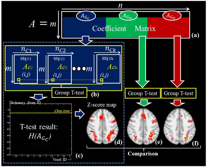
Specifically, as illustrated in Fig.2a, the A matrix can be decomposed into 3 matrices that represent three groups. As further shown in Fig.2b, each group is composed of sub-matrices of subjects, e.g., A_GC is composed of A_c1, A_c2… A_ck. As the subjects are normalized in the MNI template space and the common mask is thus employed to extract fMRI signals. So the A_n (i, j) in each sub-matrix stores the reference coefficient of the j^th voxel to the i^th component in the dictionary (Fig.2b). For each group, we hypothesize that each coefficient A_Gx (i, j) is group-wisely null, and the T-test (with T defined as Eq.(7)) is carried out to test acceptance or rejection of the null hypothesis for each element A_Gx (i, j). Note that x indicates the group category, n denotes the subject ID in each group. Here the threshold of P<0.05 is used to reject null hypothesis. The derived T-value can be easily transformed to the standard z-score (Beckmann et al., 2003).

$$\begin{array}{c}\hfill T(i,j)=\frac{\overline{A_{G_x}(i,j)}}{\sqrt{\mathit{Var}\left(A_{G_x}(i,j)\right)}∕n},A_{G_x}(i,j)=\left\{A_n\right(i,j):n=1,2,\cdots xk\}.(x=C\text{or}N\text{or}D),\hfill \\ \hfill \overline{A_{G_x}(i,j)}=\frac{1}{n}\sum _{n=1}^{xk}{A}_n(i,j),\mathit{Var}\left(A_{G_x}(i,j)\right)=\frac{1}{n}\sum _{n=1}^{xk}{\left(A_n\right(i,j)-\overline{A_{G_x}(i,j)})}^2\hfill \end{array}$$ (7)

Fig.2.

(a) A matrix is composed of three groups of subjects. (b) Correspondence of elements in A_GC and group-wise null hypothesis T-test for each element. (c) The group-wise T-test results of acceptance of null (black dots) or rejection (white dots) (P<0.05). (d) Each row in (c), which represents a network component, is mapped back to the brain volume color-coded with z-scores. (e) and (f) are z-score maps derived from G_N and G_D with the same method of (b-d).

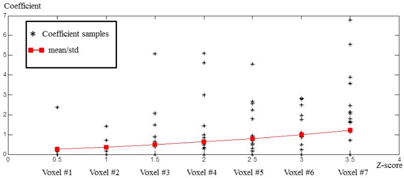
Since the dictionary learning and sparse representation constrain the sparsity of A matrix, the T-test result of A_Gx is also a sparse matrix, as shown in Fig.2c. Here, each row in the matrix of Fig.2c represents the statistically non-zero contribution in the whole brain of each dictionary atom. And each row can be mapped back to brain volume, which stands for the spatial distribution of the dictionary atom. Notably, we call each dictionary atom and the correspondence distribution a network component in this work. In order to illustrate the significance of the contribution of each network, we color-code the z-scores of each component, which is named the statistical coefficient map (SCM) here, as illustrated in Fig.2d. The T-test is carried out separately for A_GC, A_GN and A_GD, but the derived z-scores maps (such as Figs.2d-2f), which possess correspondence of the same dictionary atom, can be compared across groups. Seven examples of voxels, whose z-scores are 0.5, 1, 1.5, 2, 2.5, 3 and 3.5 in one of the statistical coefficient map of control group, are shown in Fig.3. For each example voxel, the black stars represent the coefficient value in 16 subjects, and the red block indicates the mean value of black stars divided by their standard deviation respectively. We can see that, the z-score increases with the increasing of mean/std. So, the derived z-score is an effective statistical measurement of the significance of component contribution.

Fig.3.

The coefficient distribution of 7 example voxels in 16 subjects from the control group. The z-scores of the five voxels are 0.5, 1.0, 1.5…… 3.5. For each example voxel, the black stars are coefficients from 16 subjects, and the red block indicates the mean value of the black stars divided by the standard deviation of the black stars.

Conceptually, the SCM has several key differences in comparison with the widely used statistical parametric mapping (SPM) (Beckmann et al., 2003) associated with the GLM method. First, parameters estimated from the GLM model are model driven, and regressors are pre-defined with a limited number of task paradigms. While the SCM is based on a set of group-wisely learned and optimized signal basis, and thus the abundant response patterns learned by data-driven strategy from fMRI data tend to be more effective to assess the rich information encoded in the fMRI data. Second, the SPM maps are clusters of voxels whose signal are similar to task design, the intensity of which is the significance of similarity. In comparison, the SCM maps are decomposed overlapped brain networks, the intensity of which are the significance of contribution of the network. Third, the commonly learned dictionary can effectively leverage the commonness and discrimination across subjects and groups, which makes the SCM robust to noise and comparable across subjects and groups. Fourth, the sparsity constraint regularizes the regressor selection while learning coefficient, i.e., if the regressor does not significantly contribute, the coefficient will be penalized as 0. Consequently, the results from group non-zero T-test will be stricter. As a result, SCM maps might be more reliable in measuring the significance of contribution than SPM.

3 Experimental Results

The framework has been applied on the data set of three groups of PAE related subjects: G_C, G_N and G_D (Santhanam et al., 2009). The severity of PAE is in the order of G_C<G_N <G_D (Santhanam et al., 2009). The common dictionary is learned for all three groups and the group-wise statistics in Section 2.4 was applied to each group separately. We first detected arithmetic-related networks in G_C as reported in Section 3.1 and diverse dynamic networks in Section 3.2. Further cross-group comparisons in Section 3.3 showed that group differences can be observed in these networks.

3.1 Inferred Arithmetic Related Networks

As mentioned before, with the dictionary learning and sparse coding method, a variety of networks are learned with temporal and spatial aspects of representation, namely, the time series patterns in D and the spatial maps in A. In order to interpret meaningful networks, we first compare time series patterns in D with the stimulus design, and in this way task-correlated networks and anti-task networks can be identified. On the other hand, based on the statistical coefficient maps (SCM) derived from Section 2.4 and by using the experimentally determined threshold Z>1.65, we determined voxels that have significant reference to each dictionary atom. Note that in standard z-distribution, P (Z>1.65) =0.05. We select Z>1.65 as the threshold, which is relatively lower than traditional activation analysis. That’s because our coefficient matrix is sparse, and if one network is not significantly consistent the coefficient is punished to be zero, which is a strict false positive control. Thus, with a relative low but meaningful Z threshold, we could possibly detect accurate network spatial maps. The spatial distribution of task correlated networks and anti-task networks are then explored in this section.

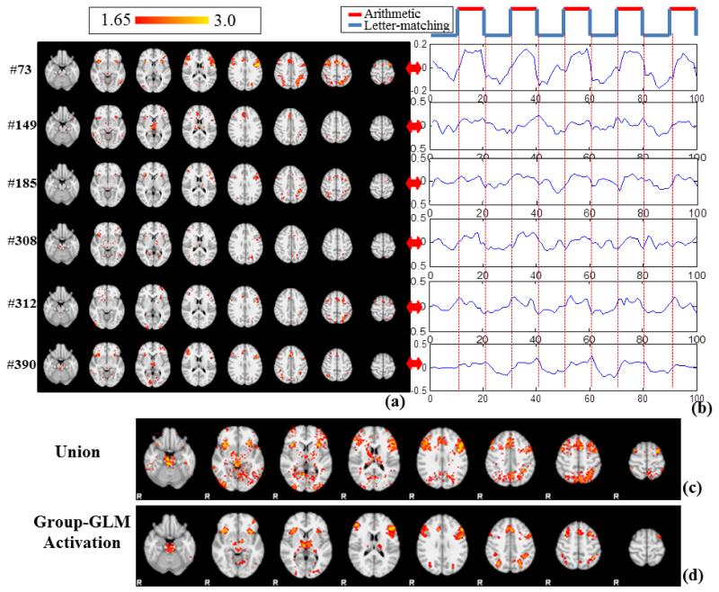
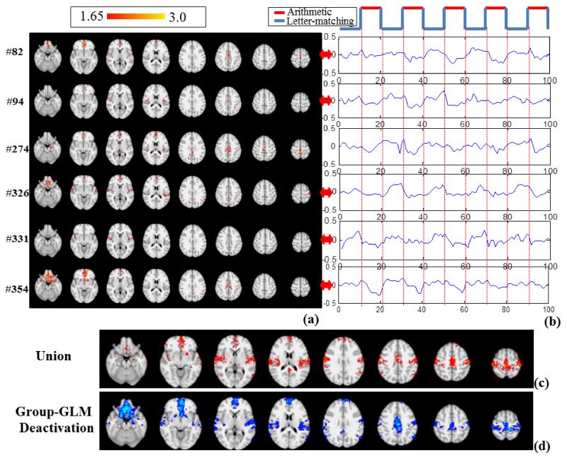
First, the task design curve as shown in the top panel of Fig.4b is convolved with the hemodynamic response function (HRF), for calculating Pearson’s correlation with all of the learned dictionary atoms. With the threshold (>0.5) and (<−0.5) applied to the correlations, 6 dominant task-correlated networks and 6 dominant anti-task networks with relatively large voxel numbers were identified, respectively, from all of the learned networks. As shown in Table 1, the peak correlation and anti-correlation could be as high as 0.813 and −0.754. In comparison, the correlations of original fMRI time series with the task stimulus curve on the volumetric voxels that exhibit the highest and lowest z-scores are shown in Table 2. It is evident that the dictionary learning method is quite sensitive in detecting task correlated and anti-task components even in the group level of large data space. For further exploration, we visualized the 6 dominant component networks from both task correlated networks and anti-task networks, whose spatial z-score maps (>1.65) and time series patterns are shown in Fig.4a-b and Fig.5a-b respectively.

Fig.4.

(a) The z-score map (Z>1.65) of the 6 networks exhibiting high correlation with task design (MNI space). (b) The corresponding signal patterns in D of the 6 network components. (c) Group-wise union of the highly task-related networks. (d) Group-wise activation detected by the GLM method (Z>3.0, cluster-correction).

Table 1.

Pearson’s correlation and anti-correlation between time series of dominant networks and HRF convolved task design.

Task Correlated	Comp. ID #	73	149	185	308	312	390	Avg.
	Correlation	0.813	0.567	0.627	0.610	0.585	0.793	0.666

Anti-Task	Comp. ID #	82	94	274	326	331	354	Avg.
	Correlation	− 0.754	−0.690	−0.579	−0.747	−0.626	−0.556	−0.659

Table 2.

(a). The Pearson’s correlations of top activated voxels from 8 subjects. As shown in the third row, the voxels exhibit the highest z-score in each subject. (b) The Pearson’s anti-correlations of top deactivated voxels from 8 subjects. The voxels exhibit the lowest z-score in each subject.

(a)
Subject	1	2	3	4	5	6	7	8	Avg.
Voxel	(26,46,12)	(32,22,2)	(30,15,3)	(45,35,23)	(49,21,10)	(41,34,24)	(46,38,15)	(48,20,9)
Z-score	6.80	6.87	6.59	9.06	7.08	6.26	10.82	7.96	7.68
Correlation	0.654	0.668	0.707	0.819	0.763	0.672	0.703	0.765	0.719

(b)
Subject	1	2	3	4	5	6	7	8	Avg.
Voxel	(30,55,10)	(31,15,26)	(33,44,11)	(36,52,18)	(43,31,19)	(31,43,12)	(31,27,32)	(34,48,14)
Z-score	−6.56	−7.37	−6.08	−7.42	−9.03	−6.35	−7.73	−8.41	−7.37
Correlation	−0.369	−0.669	−0.390	−0.695	−0.728	−0.647	−0.697	−0.436	−0.579

Fig.5.

(a) The z-score map of the 6 networks (Z>1.65) performing high anti-correlation with task design (MNI space). (b) The corresponding signal patterns in D of the 6 network components. (c) Group-wise union of the highly anti-task networks. (d) Group-wise de-activation detected by the GLM method (Z<−3.0, cluster-correction).

In comparison with the group-wise activation detection from the GLM method (Fig.4d), the networks detected by our approach exhibit multiple task-activated patterns. Notably, the shape differences among these temporal patterns separated the generally defined activations by GLM into sub-networks. For instance, the sub-networks in Fig.4a serve as parts of the activation patterns in Fig.4d. If we simply aggregated all the 6 task correlated maps (by a union operation) and name it as the “Union” of task correlated networks, as shown in Fig.4c, the spatial pattern (Fig.4c) is quite similar as the activation pattern in Fig.4d. In order to quantitatively measure how much our networks cover the activation map, we calculated the true positive rate (TPR) or sensitivity as:

$$\mathit{TPR}=\frac{{\mathit{SM}}_{◠}T}{T}$$ (8)

where SM is the spatial map of our inferred networks/sub-networks and T is the spatial map of the group-wise activation pattern in Fig.4d, which is treated as a template here. The TPR is measured for each sub-network in Table 3 as well as the “Union” of networks. We can observe that these networks cover the activation map by GLM differently, and the most dominant component #73 cover as high as 0.745 of the GLM-based activation. It is interesting that their union of our inferred sub-networks cover about 0.926 of the GLM-based activation. Similar qualitative and quantitative comparisons are also performed for the anti-task networks as shown in Fig.5 and Table 3. The union of the anti-task networks exhibit 0.817 TPR of the GLM-based deactivation map in Fig.5d. On the other hand, it is essential to inspect if these networks are highly overlapped, i.e., if these networks are spatially independent. Note that, TPR does not apply anymore in this situation, because it is uneven to treat any network as a template. Thus, Jaccard similarity is employed to calculate the overlap rate (OR) as defined in Eq.(9) to measure the overlap between task correlated networks and anti-task networks respectively. In Eq.(9), N_a and N_b are spatial maps of two networks. The overlap rate is defined by the intersection of two networks divided by their union.

$$\mathit{OR}=\frac{{N_a}_{◠}{N}_b}{{N_a}_{◡}{N}_b}$$ (9)

Table 3.

The true positive rate (TPR) of task correlated network components, anti-task components and their union respectively in the group-wise activation and deactivation maps.

Task	CompID	#73	#149	#185	#308	#312	#390	Union
	TPR	0.745	0.209	0.393	0.132	0.091	0.434	0.926

Anti- Task	CompID	#82	#94	#274	#326	#331	#354	Union
	TPR	0.376	0.068	0.133	0.214	0.049	0.632	0.817

In the results shown in Table 4, as we can see that the overlap between these task-correlated/anti-task networks are quite small, e.g., the average overlap is 0.05 for task correlated networks and is 0.036 for the anti-task networks. From these results, it is evident that the task-related and anti-task sub-networks inferred by our method are relatively spatial independent.

Table 4.

(a) The spatial overlap ratio (OR) among the 6 task correlated networks. (b) The spatial overlap ratio (OR) among the 6 anti-task networks.

(a)
OR	#73	#149	#185	#308	#312	#390
#73	1.000	0.032	0.161	0.030	0.088	0.107
#149		1.000	0.025	0.017	0.014	0.054
#185			1.000	0.021	0.060	0.088
#308				1.000	0.008	0.023
#312					1.000	0.018
#390						1.000

(b)
OR	#82	#94	#274	#326	#331	#354
#82	1.000	0.037	0.086	0.071	0.083	0.092
#94		1.000	0.039	0.022	0.015	0.018
#274			1.000	0.030	0.002	0.026
#326				1.000	0.030	0.053
#331					1.000	0.009
#354						1.000

Additionally, the anatomical distribution of the union of sub-networks (Fig.4c and Fig.5c) detected by our method is in agreement with the results in the previous work (Santhanam et al., 2009; Santhanam et al., 2011). Task correlated networks are quite consistent with the activation detected in the previous study (Santhanam et al., 2009), including regions of bilateral parietal lobe, medial frontal gyrus, and bilateral middle frontal gyrus, which are also shown in Fig.4d. These regions have been shown to be related to arithmetic and working memory (Santhanam et al., 2009). Also, the anatomical distribution of the union of deactivation sub-networks by our methods, including the MPFC and the PCC, is akin to the previous report (Santhanam et al., 2011), as shown in Fig. 5d. In summary, our method is capable of detecting multiple meaningful task-related and anti-task sub-networks, the total of which are in agreement with the GLM-based group-wise activation. However, our method can provide much more details about the temporally and spatially different sub-networks. The interpretation of neuroscientific meanings of such variety of sub-networks entails more effort in the future.

3.2 Diverse Dynamic Networks

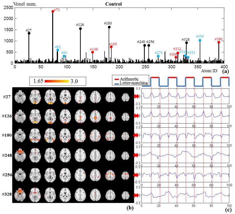
In addition to the sub-networks identified in Section 3.1, other sub-networks that include dominant number of voxels are also explored in this section. Through frequency analysis on these networks, we observed diverse network dynamics other than traditionally conceived activations and deactivations. Specifically, by thresholding all of the statistical coefficient maps (SCMs) in the control group using Z>1.65, we count the remaining voxel numbers in Fig.6a. The task correlated networks and anti-task networks are marked with red and blue respectively, from which we can see that some of them include dominant numbers of voxels while some of them do not. Apart from the red and blue marks, there are also certain networks that contain dominant numbers of voxels, e.g., # 27, #126 and #180. We picked up 6 most dominant networks and visualized their spatial maps and temporal patterns in Figs.6b-6c. In Fig.6b, these networks are mainly located on the visual cortex, part of the default mode network and subcortical areas. The Pearson’s correlations with task design curve of these networks are relatively low, as shown in Table 5. By inspecting their time series patterns in Fig.6c, it is interesting that the network components of #27, #126, #180 and #256 exhibit high positive or negative impulses at the task change points. While #248 shows magnitude increase in letter-matching task and magnitude decrease in arithmetic task. Also, #328 is similar to anti-correlation pattern but it involves more uncertain fluctuations. The periodical reactions of all these networks exhibit high relevance to the task design curve, though they have quite diverse dynamics. This might be the reason that they are overlooked by the GLM based activation detection, and thus we call them diverse dynamic networks (DDN) in this paper.

Fig.6.

(a) Voxel number histogram of the 400 network components in the control group. Here, the highly task related networks in Fig.4 are marked with red color and the highly anti-task networks in Fig.5 are marked with blue color. Six dominant networks with high voxel numbers are marked with black. (b) The z-score map of the 6 networks (Z>1.65) marked with black color in (a). (c) The corresponding signal patterns in D of the 6 network components.

Table 5.

The Pearson’s correlations between the time series of diverse dynamic networks (DDN) and HRF-convolved task design curve.

DDN	Comp. ID #	#27	#126	#180	#248	#256	#328
	Correlation	0.239	−0.031	0.170	−0.265	0.043	−0.411

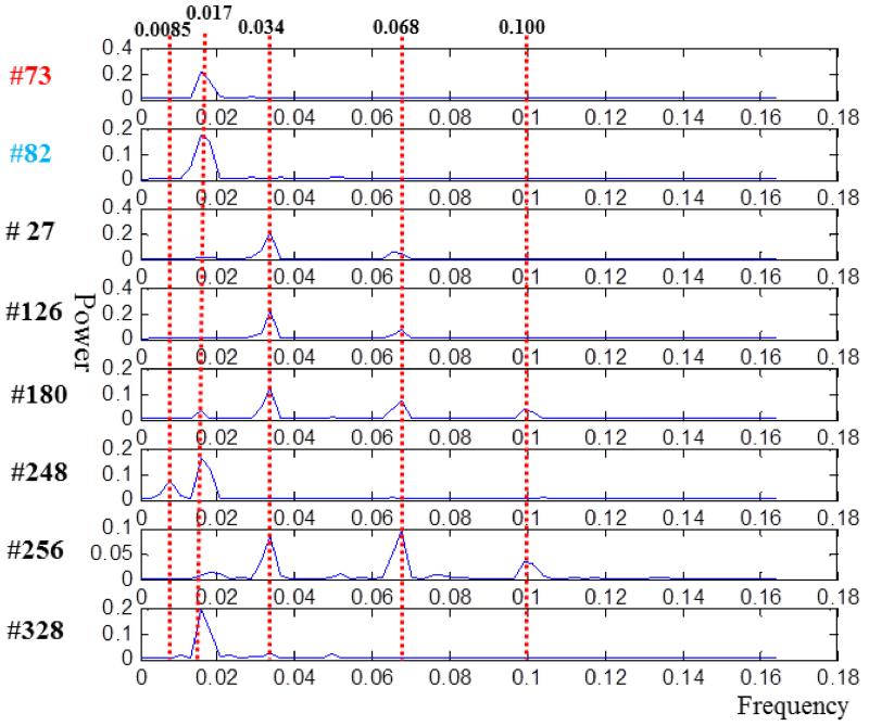
To further explore the diverse dynamic networks (DDNs), we applied the Fourier transform to the time series of the corresponding dictionary network atoms, as shown in Fig.7. For comparison, the power distributions of task correlated network #73 and anti-task network #82 are also shown in the top panels of Fig.7. Since TR=3s and the period of a task cycle is 20 TRs, the task frequency is 1/(20×3s)=0.017 HZ. The power of task and anti-task networks are also concentrated on the task frequency of 0.017 HZ, as expected. But the diverse dynamic networks exhibited multiple frequencies. As shown in Fig.7, the power of network #27, #126, #180 and #256 are mostly concentrated at doubled task frequencies (around 0.034 HZ) or four times of task frequency (around 0.068 HZ). The network components #180 and #256 even have peaks at six times of task frequency (around 0.100 HZ). The networks components #248 and #328 are concentrated on the task frequency, but low frequency energy at around 0.0085 HZ also contributes to the signal pattern of #248 and there are other frequencies in #328. These diverse dynamic networks provide evidence that there are multiple frequency responses in the human brain to tasks, and a certain brain region might exhibit multi-frequency responses. Also, these multi-frequency responses cannot be effectively detected by the traditional GLM-based method. These responses might occur at the brain areas that are not directly responsible for arithmetic or working memory but are believed to contribute to information input and attention regularization, such as the visual cortex, default model network or subcortical areas. In summary, the detection and characterization of these diverse dynamic networks demonstrated the advantage of our dictionary learning and sparse coding based framework.

Fig.7.

The power distribution across frequencies of diverse dynamic networks in Fig.6c after applying Fourier transform.

3.3 Effects of PAE

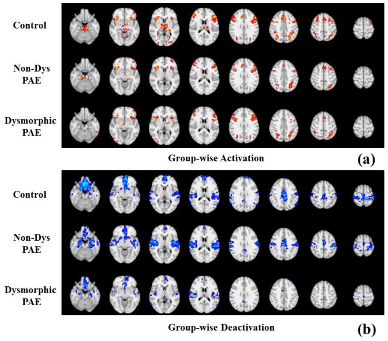
As reported in the literature (Santhanam et al., 2009; Santhanam et al., 2011), the activation and deactivation regions tend to shrink with the increment of severity of PAE effect. We repeated the GLM based group-wise activation and deactivation detection with the FSL toolbox (Beckmann et al., 2003), and similar results are achieved, as shown in Fig.8 and Table 6. In this session, we will explore if the size of statistical coefficient maps (SCM) will be affected by the severity of PAE.

Fig.8.

Comparison of activation maps (Z>3.0) and deactivation maps (Z<−3.0) from three groups of subjects by repeating GLM based group-wise activation and de-activation.

Table 6.

Voxel numbers of group-wise activation regions and deactivation from GLM based method in three groups by using different levels of threshold. The activation using threshold Z>3.0 and deactivation using threshold Z<−3.0 are visualized in Fig.8.

Activation	Control	Non-Dys PAE	Dysmorphic PAE
Z>2.5	4906	3096	3057
Z>3.0	2630	1373	1276
Z>3.5	1103	461	437
Z>4.0	364	113	100

Deactivation	Control	Non-Dys PAE	Dysmorphic PAE
Z<−2.5	6163	5955	2484
Z<−3.0	3100	3098	787
Z<−3.5	1315	1165	148
Z<−4.0	487	241	18

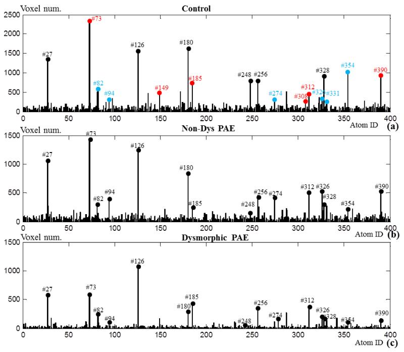
First, we compare the voxel number histograms of all statistical coefficient maps from three groups of subjects including controls, exposed non-dysmorphic PAE (Non-Dys PAE) and exposed dysmorphic PAE (Dysmorphic PAE) in Fig.9a-9c based on the correspondence established by the common dictionary D. The same threshold of Z>1.65 is chosen for all networks from three groups. Globally, the voxel number distribution is quite similar across three groups, especially the marked dominant networks. Notably, the decreasing trend of voxel number can be observed with increment of severity of PAE, e.g., the task-correlated network #73 includes around 2300 voxels in the control group, but it only includes around 1500 voxels in the Non-Dys PAE group and only around 600 voxels in the Dysmorphic PAE group.

Fig.9.

Voxel number histogram of the 400 network components in the three groups of Control, Non-dys PAE and Dysmorphic PAE groups, respectively. (a) is the same as Fig.6a.

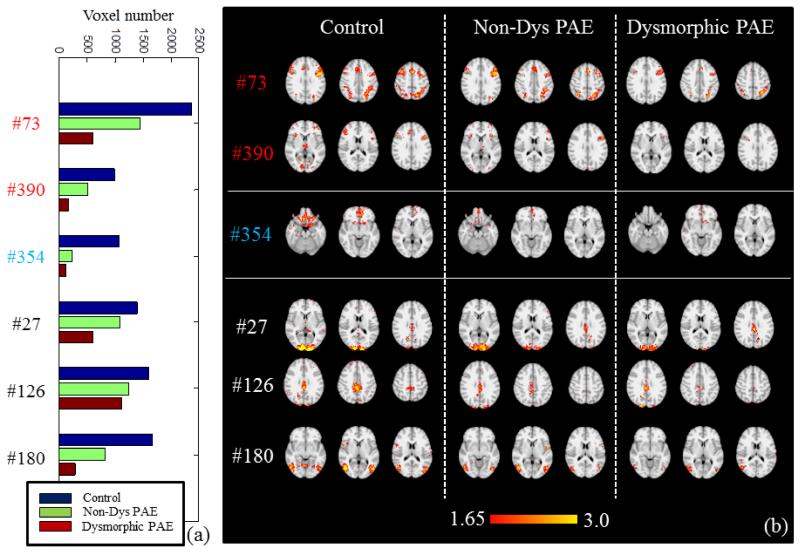
After sorting the voxel number of each corresponding network in three groups, it can be found that the size of most of the networks decreases with the increment of severity of PAE. We visualize the 6 most dominant networks in Fig.10. Histogram of voxel numbers are shown in Fig.10a, and the decreasing trend is quite evident. Also, the diminution is observable from the spatial maps in Fig.10b. Among these 6 networks, #73 and #390 are categorized into task correlated networks, #354 is considered as an anti-task network, and #27, #126 and #180 are believed to be three diverse dynamic networks, as discussed in Section 3.2. The diminution of task-related networks include the left superior and right inferior parietal regions and the medial frontal gyrus, which is in agreement with the activation detection in our work and previous work in Santhanam et al., 2009. The diminution of anti-task network includes sub-cortical areas and MPFC, and this concurs with previous work as well (Santhanam et al., 2011). It is interesting that the diverse dynamic networks, including visual cortex and default mode network, also shrink with the more severity of PAE.

Fig.10.

Six networks whose voxel number is in decreasing order across three groups, i.e., V(Control)>V(Non-Dys PAE)>V(Dys PAE). (a) Voxel number (P<0.05, Z>1.65) comparison of the 6 networks from three groups. (b) The z-score map comparison of 6 networks from three groups.

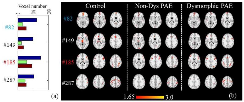
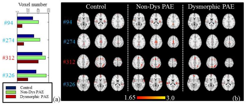
Apart from the dominant networks shown in Fig.10, we can also find some other minor networks that include less numbers of voxels. The network sizes exhibit different patterns of relationship with the severity of PAE, as shown in Fig.11-12. In Fig.11a-11b, networks in the control group have the highest voxel sizes, while the Dysmorphic group has intermediate sizes and the Non-Dys group has the lowest. In contrast, for the networks in Fig.12a-12b, the Non-Dys group has the highest activation, the control group performs intermediately, and the Dysmorphic group has the lowest. Most of these networks are considered as anti-task networks, and it is evident that PAE effect might not be necessarily linear to certain brain networks. This effect needs more future interpretation, but it is inspiring that they can be captured by our group-wise sparse coding method.

Fig.11.

Four networks whose voxel number is in the order of V(Control)>V(Dys PAE) )>V(Non-Dys PAE) across three groups. (a) Voxel number (P<0.05, Z>1.65) comparison of the 4 networks from three groups. (b) The z-score map comparison of 4 networks in (a) from three groups.

Fig.12.

Four networks whose voxel number is in the order of V(Non-Dys PAE)>V(Control)>V(Dys PAE) across three group. (a) Voxel number (P<0.05, Z>1.65) comparison of the 4 networks from three groups. (b) The z-score map comparison of 4 networks in (a) from three groups.

4 Reproducibility Analysis

4.1 Simulation Experiment

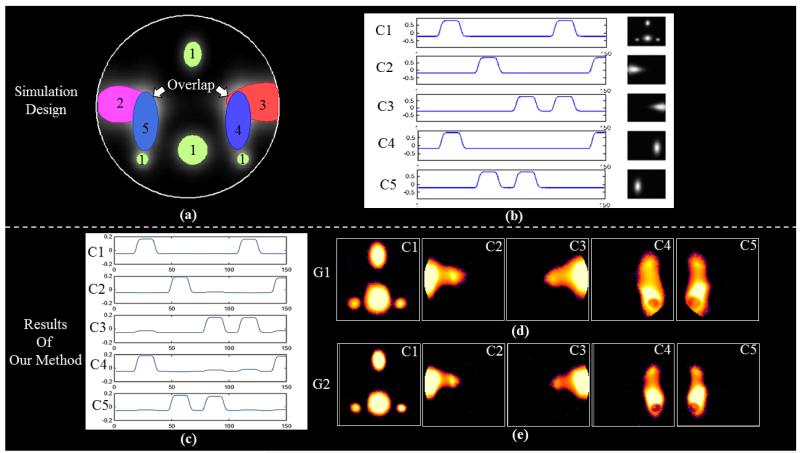
To validate the effectiveness of our method on multiple group analysis, we designed an experiment based on the fMRI simulation toolbox SimTB (http://mialab.mrn.org/software; Erhardt et al., 2012). Specifically, as shown in Fig.13 five components are simulated in two comparable groups (10 subjects in each). The spatial shapes of the components are shown in Fig.13a, and overlaps are designed between component 2 and 5, and between component 3 and 4. Block designed signals convolved by canonical HRF are visualized in Fig.13b. Inter-subject variability are simulated by 1~3 voxel (uniformly distributed) x-translation, 1~3 voxel (uniformly distributed) y-translation, and 1~5 degrees (uniformly distributed) rotation. Cross-group difference are realized by different component sizes, i.e., the sizes of components in the subjects of Group 1 is 1.3~1.5 times (uniformly distributed) larger than that of Group 2. Rician noise is added to each simulated subjects with the contrast-to-noise ratio of 1~3 (uniformly distributed).

Fig.13.

Simulation experiment with simulation toolbox SimTB (http://mialab.mrn.org/software). (a) The spatial layout of the five simulated components. There are overlaps between C2 and C5, and between C3 and C4. (b) The simulated signal patterns of the five components. Two comparable groups of subjects are simulated. The average component sizes of Group 2 is smaller than Group1. (c) The learned signal patterns of the five components from two groups using our method. (d) The spatial patterns of SCMs from Group 1. (e) The spatial patterns of SCMs from Group 2.

With our proposed method, we learn the common signal pattern dictionary from the two groups of subjects. Since we already know the component number, we set the dictionary size as 5. As visualized in Fig.13c, the simulated signals of components are well reconstructed. The SCMs are calculated for each component of each group and are shown in Fig.13d and 13e. Since the simulation is based on very easy assumption, the significance of components could be high, so that we choose Z-threshold as 2.0. We can see that, the spatial maps of components from both groups are reconstructed, especially the component 1 with multiple regions. Also the components (2, 5, 3, 4) with overlaps are well recovered. Additionally, comparing Fig.13d and Fig.13e, the size difference of components between two groups are detected as designed, i.e., the SCMs of Group 1 are obviously larger than that of Group 2. Based on the simulation, we can conclude that our method is effective in reconstructing overlapped component networks from multiple groups, and is capable of capturing group-wise differences at the network level.

4.2 Reproducibility with Different Dictionary Size

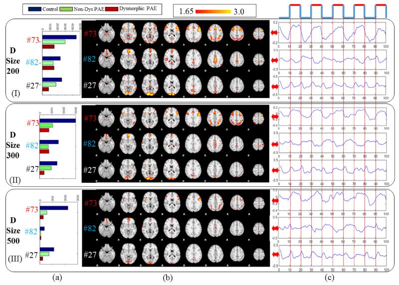
Dictionary size is an important parameter of dictionary learning and sparse coding. In our paper we experimentally determine the dictionary size as 400. However, we also tried the dictionary size of 200, 300 and 500. Based on our experiments, we found that by increasing the dictionary size, the detected networks might decrease in size. Firstly, that’s because the coefficients might be diluted by more dictionary atoms. And another reason is that it’s possible that one network will be decomposed into multiple component networks or similar networks. So in this paper, on the purpose of balancing dictionary size and network diversity we determine the dictionary size as 400. But as shown in Fig.14, with dictionary size set as 200, 300 and 500 the dominant task-related network, anti-task network and diverse dynamic network could always be detected. And the spatial patterns (Fig.14b) and temporal patterns (Fig.14c) are quite consistent across different dictionary sizes. From Fig.14a, we also found that the group difference can also be consistently detected with different dictionary settings, i.e., the sizes of network #73 and #27 decrease with the increment of PAE severity and the size of network #82 follow the pattern of V(Control)>V(Dys PAE))>V(Non-Dys PAE). In summary, we conclude that although the dictionary size might impact the network size and diversity, the representative networks could be consistently reproduced with different dictionary size setting. And the group differences could also be consistently captured by our method. In summary, our method is reliable and reproducible.

Fig.14.

Reproducibility experiment with different dictionary size. Block (I) (II) (III) represent three dominant networks detected by setting of dictionary size as 200, 300 and 500, respectively. #73 is a task-related network, #82 is an anti-task network and #27 is a diverse dynamic network. (b) The voxel number of the networks in three groups. (b) The spatial maps of the three networks. (c) The signal pattern of the three networks.

5 Discussion and Conclusion

5.1 Overview

In this paper, we have presented a novel group-wise sparse representation and statistical coefficient mapping (SCM) approach for analyzing multiple populations with task fMRI data. The aggregated task fMRI signals from multi-groups of subjects are systematically represented as a learned common collection of signal basis and their spatial coefficient distribution maps. Temporal and frequency analysis on the dictionary basis elucidated the diversity of task evoked activity patterns. Statistical assessment of the spatial maps across subjects and inter-group comparison provide fine-granularity perspectives of detecting discriminations between brain conditions and normal controls. The approach has been applied on three groups of subjects which are affected by PAE in different degrees. Experimental results have suggested that our data-driven group-wise method can detect diverse task-related brain networks simultaneously, and these networks consistently exist across three groups but are affected in different ways with the increment of severity of PAE.

5.2 Methodological Advantage

The methodological advantages of our sparse coding and statistical coefficient mapping (SCM) are summarized as follows. First, the group-wise common dictionary bases are learned and optimized from the whole fMRI data, which consist of abundant response patterns. Thus, they are more adaptive to neurophysiology specification, more systematic in discovering diverse brain networks, and more sufficient in assessing rich information encoded in the whole fMRI data than the traditional GLM method. Second, the commonly learned dictionary can effectively leverage the commonness and discrimination across subjects and groups, which makes the SCM more robust to noise and more powerful in detecting cross-group differences, which is greatly preferred by systematic clinical assessment, such as PAE. Third, the sparsity constraint regularizes the regressor selection while learning coefficient, consequently the results from group non-zero T-test will be more strict. As a result, SCM maps are more reliable in measuring the significance of contribution. Finally, in comparison with previous sparse representation of fMRI signals of each individual brains for network analysis (Lee et al., 2011; Lv et al., 2014b), our group-wise statistical method can automatically establish their correspondences across different populations and systematically assess the functional activity differences among these populations. Correspondence of individual component networks is established by learning the common dictionary basis from multiple groups and subjects, and the spatial normalization of individual brains and signal extraction guided by the common mask provides a foundation for statistical analysis and inter-group comparison.

5.3 The Robustness of the Method

Sparsity, which is a major feature of our method, take the responsibility of detecting statistically robust networks. In our method, the fMRI signal of each voxel from each subject was sparsely represented by the learned and optimized common signal basis. If one dictionary atom is not relevant to the certain signal, the corresponding coefficient will be penalized to zero. In other words, the sparse constraint regularizes the signal basis selection. Consequently, most elements of the coefficient matrix are zeros. Thus, the voxels survived from T-test in the SCMs have to be substantially and consistently non-zero. That’s the reason that most SCMs perform very low voxel number as shown in Fig.9. And it is exactly in this way, that the sparsity guaranteed the robustness of the networks.

The common dictionary learning from multiple groups of subjects make our method less sensitive to noises such as motions. Most of the noises are individually specified, but the dictionary is learned to represent common features across groups of subjects. Thus, either the noises would be dropped in the residuals of sparse representation or be learned as dictionary atoms if the dictionary is big enough.

Additionally, the learned activation signal patterns are more adaptive and flexible in the perspective of hemodynamic function as shown in Fig.4b. While in traditional GLM method, the hemodynamic function are usually pre-defined and uniformed for the whole brains of different subjects. And it’s evident that in Fig.4, different activated brain regions might perform different hemodynamic functions. Therefore, our method is also robust to hemodynamic variation.

5.4 Improvement of Analysis

Our proposed method was applied on the same data set of Santhanam et al. (2009). The major contribution of Santhanam et al. (2009) is the finding of diminution of activation and de-activation relevant to the severity of PAE. In comparison, our method not only detect this kind of diminution in activation/de-activation, but also refine the results in multiple activated or de-activated networks, which perform adaptive task-related signal patterns. In addition, we also found the diminution is present in multiple diverse networks, which have not yet been detected by traditional methods. However, in our work, we also captured that diminution is not the only pattern that applies to all networks. As shown in Fig.11 and Fig.12, different patterns could be found regarding the effect of PAE.

5.5 Challenges and Future Work

However, there are also challenges associated with this novel computational framework. First, there is little neuroscience evidence regarding how many component networks should be decomposed for the group of task fMRI signal sets so far. As a result, it is difficult to determine the learned dictionary size theoretically. Instead, our current results were based on experimentally determined network number. It will be one of our major future works to optimize the network number. Second, due to the lack of ground truth in fMRI, it is difficult to interpret the neuroscience meaning of all the learned hundreds of brain networks. Thus, more temporal, frequency and spatial characterization methods should be developed in the near future for better interpretation of our results. Finally, this novel framework should be applied in other task fMRI datasets of brain conditions and controls, in order to examine its reproducibility and robustness. It is believed that this framework would find many applications in clinical and cognitive neurosciences in the future.

Highlights.

1. Novel approach of group-wise sparse representation of the fMRI data.

2. Assess the systematic functional activity differences among three populations.

3. A collection of brain networks affected by different levels of severity of prenatal alcohol exposure.

References

- Abolghasemi V, Ferdowsi S, Sanei S. Fast and incoherent dictionary learning algorithms with application to fMRI. Signal, Image and Video Processing. 2013;9(1):147–158. [Google Scholar]
- Ardekani BA, Kanno I. Statistical methods for detecting activated regions in functional MRI of the brain. Magnetic Resonance Imaging. 1998;16(10):1217–1225. doi: 10.1016/s0730-725x(98)00125-8. [DOI] [PubMed] [Google Scholar]
- Andersen AH, Gash DM, Avison MJ. Principal component analysis of the dynamic response measured by fMRI: a generalized linear systems framework. Magnetic Resonance Imaging. 1999;17(6):795–815. doi: 10.1016/s0730-725x(99)00028-4. [DOI] [PubMed] [Google Scholar]
- Bandettini PA, Jesmanowicz A, Wong EC, Hyde JS. Processing strategies for time-course data sets in functional MRI of the human brain. Magnetic Resonance in Medicine. 1993;30(2):161–173. doi: 10.1002/mrm.1910300204. [DOI] [PubMed] [Google Scholar]
- Baumgartner R, Scarth G, Teichtmeister C, Somorjai R, Moser E. Fuzzy clustering of gradient-echo functional MRI in the human visual cortex. Part I: Reproducibility. Journal of Magnetic Resonance Imaging. 1997;7(6):1094–1101. doi: 10.1002/jmri.1880070623. [DOI] [PubMed] [Google Scholar]
- Beckmann CF, Jenkinson M, Smith SM. General multilevel linear modeling for group analysis in FMRI. Neuroimage. 2003;20(2):1052–1063. doi: 10.1016/S1053-8119(03)00435-X. [DOI] [PubMed] [Google Scholar]
- Bowman DF, Caffo B, Bassett SS, Kilts C. Bayesian hierarchical framework for spatial modeling of fmri data. NeuroImage. 2008;39:146–156. doi: 10.1016/j.neuroimage.2007.08.012. [DOI] [PMC free article] [PubMed] [Google Scholar]
- Bullmore E, Fadili J, Breakspear M, Salvador R, Suckling J, Brammer M. Wavelets and statistical analysis of functional magnetic resonance images of the human brain. Statistical Methods in Medical Research. 2003;12(5):375–399. doi: 10.1191/0962280203sm339ra. [DOI] [PubMed] [Google Scholar]
- Calhoun VD, Liu J, Adali T. A review of group ICA for fMRI data and ICA for joint inference of imaging, genetic, and ERP data. Neuroimage. 2009;45(1):S163–S172. doi: 10.1016/j.neuroimage.2008.10.057. [DOI] [PMC free article] [PubMed] [Google Scholar]
- Coles CD, Brown RT, Smith IE, Platzman KA, Erickson S, Falek A. Effects of prenatal alcohol exposure at school age. I. Physical and Cognitive Development. Neurotoxicology and Teratology. 1991;13(4):357–367. doi: 10.1016/0892-0362(91)90084-a. [DOI] [PubMed] [Google Scholar]
- Costafreda SG. Pooling fMRI data: meta-analysis, mega-analysis and multi-center studies. Frontiers in Neuroinformatics. 2009;3:33. doi: 10.3389/neuro.11.033.2009. [DOI] [PMC free article] [PubMed] [Google Scholar]
- Deng F, Zhu D, Lv J, Guo L, Liu T. FMRI Signal Analysis Using Empirical Mean Curve Decomposition. Biomedical Engineering, IEEE Transactions on. 2013;60(1):42–54. doi: 10.1109/TBME.2012.2221125. [DOI] [PMC free article] [PubMed] [Google Scholar]
- Derrfuss J, Mar RA. Lost in localization: The need for a universal coordinate database. NeuroImage. 2009;48(1):1–7. doi: 10.1016/j.neuroimage.2009.01.053. [DOI] [PubMed] [Google Scholar]
- Descombes X, Kruggel F, Von Cramon DY. fMRI signal restoration using a spatio-temporal markov random field preserving transitions. NeuroImage. 1998;8(4):340–349. doi: 10.1006/nimg.1998.0372. [DOI] [PubMed] [Google Scholar]
- Duncan J. The multiple-demand (MD) system of the primate brain: mental programs for intelligent behaviour. Trends in Cognitive Sciences. 2010;14(4):172–179. doi: 10.1016/j.tics.2010.01.004. [DOI] [PubMed] [Google Scholar]
- Erhardt EB, Allen EA, Wei Y, Eichele T, Calhoun VD. SimTB, a simulation toolbox for fMRI data under a model of spatiotemporal separability. Neuroimage. 2012;59(4):4160–4167. doi: 10.1016/j.neuroimage.2011.11.088. [DOI] [PMC free article] [PubMed] [Google Scholar]
- Friston KJ, Holmes AP, Worsley KJ, Poline JP, Frith CD, Frackowiak RS. Statistical parametric maps in functional imaging: a general linear approach. Human Brain Mapping. 1994;2(4):189–210. [Google Scholar]
- Gazzaugia MS, editor. The Cognitive Neurosciences III. The MIT Press; 2004. [Google Scholar]
- Hamilton AF. Lost in localization: A minimal middle way. Neuroimage. 2009;48:8–10. doi: 10.1016/j.neuroimage.2009.05.007. [DOI] [PubMed] [Google Scholar]
- Hartvig NV, Jensen JL. Spatial mixture modeling of fmri data. Human Brain Mapping. 2000;11(4):233–248. doi: 10.1002/1097-0193(200012)11:4<233::AID-HBM10>3.0.CO;2-F. [DOI] [PMC free article] [PubMed] [Google Scholar]
- Heeger DJ, Ress D. What does fMRI tell us about neuronal activity? Nature Reviews Neuroscience. 2002;3(2):142–151. doi: 10.1038/nrn730. [DOI] [PubMed] [Google Scholar]
- Huaien L, Puthusserypady S. fMRI data analysis with nonstationary noise models: a Bayesian approach. Biomedical Engineering, IEEE Transactions on. 2007;54:1621–1630. doi: 10.1109/TBME.2007.902591. [DOI] [PubMed] [Google Scholar]
- Jenkinson M, Smith S. A global optimisation method for robust affine registration of brain images. Medical Image Analysis. 2001;5(2):143–156. doi: 10.1016/s1361-8415(01)00036-6. [DOI] [PubMed] [Google Scholar]
- Laird AR, Eickhoff SB, Kurth F, Fox PM, Uecker AM, Turner JA, Robinson JL, Lancaster JL, Fox PT. ALE meta-analysis workflows via the BrainMap database: Progress towards a probabilistic functional brain atlas. Neuroinformatics. 2009;3(23):11. doi: 10.3389/neuro.11.023.2009. [DOI] [PMC free article] [PubMed] [Google Scholar]
- Lee K, Tak S, Ye JC. A data-driven sparse GLM for fMRI analysis using sparse dictionary learning with MDL criterion. Medical Imaging, IEEE Transactions on. 2011;30(5):1076–1089. doi: 10.1109/TMI.2010.2097275. [DOI] [PubMed] [Google Scholar]
- Logothetis NK. What we can do and what we cannot do with fMRI. Nature. 2008;453(7197):869–878. doi: 10.1038/nature06976. [DOI] [PubMed] [Google Scholar]
- Li Y, Namburi P, Yu Z, Guan C, Feng J, Gu Z. Voxel selection in FMRI data analysis based on sparse representation. Biomedical Engineering, IEEE Transactions on. 2009;56(10):2439–2451. doi: 10.1109/TBME.2009.2025866. [DOI] [PubMed] [Google Scholar]
- Li Y, Long J, He L, Lu H, Gu Z, Sun P. A Sparse Representation-Based Algorithm for Pattern Localization in Brain Imaging Data Analysis. PLoS ONE. 2012;7(12):e50332. doi: 10.1371/journal.pone.0050332. [DOI] [PMC free article] [PubMed] [Google Scholar]
- Lv J, Li X, Zhu D, Jiang X, Zhang X, Hu X, Zhang T, Guo L, Liu T. Sparse Representation of Group-Wise FMRI Signals; Medical Image Computing and Computer-Assisted Intervention–MICCAI 2013; Springer Berlin Heidelberg. 2013; pp. 608–616. [DOI] [PubMed] [Google Scholar]
- Lv J, Guo L, Zhu D, Zhang T, Hu X, Han J, Liu T. Group-wise FMRI Activation Detection on DICCCOL Landmarks. Neuroinformatics. 2014a;12(4):513–534. doi: 10.1007/s12021-014-9226-5. [DOI] [PMC free article] [PubMed] [Google Scholar]
- Lv J, Jiang X, Li X, Zhu D, Zhang S, Zhao S, Chen H, Zhang T, Han J, Ye J, Guo L, Liu T. Holistic Atlases of Functional Networks and Interactions Reveal Reciprocal Organizational Architecture of Cortical Function. Biomedical Engineering, IEEE Transactions on. 2014b;62(4):1120–1131. doi: 10.1109/TBME.2014.2369495. [DOI] [PubMed] [Google Scholar]
- Lv J, Jiang X, Li X, Zhu D, Chen H, Zhang T, Zhang S, Hu X, Han J, Huang H, Zhang J, Guo L, Liu T. Sparse representation of whole-brain fMRI signals for identification of functional networks. Medical Image Analysis. 2015;20(1):112–134. doi: 10.1016/j.media.2014.10.011. [DOI] [PubMed] [Google Scholar]
- Mairal J, Bach F, Ponce J, Sapiro G. Online learning for matrix factorization and sparse coding. The Journal of Machine Learning Research. 2010;11:19–60. [Google Scholar]
- McKeown MJ, Jung TP, Makeig S, Brown G, Kindermann SS, Lee TW, Sejnowski TJ. Spatially independent activity patterns in functional MRI data during the Stroop color-naming task. Proceedings of the National Academy of Sciences. 1998;95(3):803–810. doi: 10.1073/pnas.95.3.803. [DOI] [PMC free article] [PubMed] [Google Scholar]
- Matthews P, Jezzard P. Functional magnetic resonance imaging. Journal of Neurology, Neurosurgery & Psychiatry. 2004;75(1):6–12. [PMC free article] [PubMed] [Google Scholar]
- Ng B, Abugharbieh R, Hamarneh G. Group MRF for fMRI activation detection; Computer Vision and Pattern Recognition (CVPR), IEEE Conference on; 2010.pp. 2887–2894. [Google Scholar]
- Oikonomou VP, Blekas K, Astrakas L. A sparse and spatially constrained generative regression model for fMRI data analysis. Biomedical Engineering, IEEE Transactions on. 2012;59(1):58–67. doi: 10.1109/TBME.2010.2104321. [DOI] [PubMed] [Google Scholar]
- Pessoa L. Beyond brain regions: Network perspective of cognition-emotion interactions. Behavioral and Brain Sciences. 2012;35(03):158–159. doi: 10.1017/S0140525X11001567. [DOI] [PubMed] [Google Scholar]
- Santhanam P, Li Z, Hu X, Lynch ME, Coles CD. Effects of prenatal alcohol exposure on brain activation during an arithmetic task: an fMRI study. Alcoholism: Clinical and Experimental Research. 2009;33(11):1901–1908. doi: 10.1111/j.1530-0277.2009.01028.x. [DOI] [PMC free article] [PubMed] [Google Scholar]
- Santhanam P, Coles CD, Li Z, Li L, Lynch ME, Hu X. Default mode network dysfunction in adults with prenatal alcohol exposure. Psychiatry Research: Neuroimaging. 2011;194(3):354–362. doi: 10.1016/j.pscychresns.2011.05.004. [DOI] [PMC free article] [PubMed] [Google Scholar]
- Schöpf V, Windischberger C, Robinson S, Kasess CH, Fischmeister FP, Lanzenberger R, Albrecht J, Kleemann AM, Kopietz MW, Moser E. Model-free fMRI group analysis using FENICA. Neuroimage. 2011;55(1):185–193. doi: 10.1016/j.neuroimage.2010.11.010. [DOI] [PubMed] [Google Scholar]
- Shimizu Y, Barth M, Windischberger C, Moser E, Thurner S. Wavelet-based multifractal analysis of fMRI time series. Neuroimage. 2004;22:1195–1202. doi: 10.1016/j.neuroimage.2004.03.007. [DOI] [PubMed] [Google Scholar]
- Smith SM, Jenkinson M, Woolrich MW, Beckmann CF, Behrens TE, Johansen-Berg H, Bannister PR, De Luca M, Drobnjak I, Flitney DE, Niazy RK, Saunders J, Vickers J, Zhang Y, De Stefano N, Brady JM, Matthews PM. Advances in functional and structural MR image analysis and implementation as FSL. Neuroimage. 2004;23:S208–S219. doi: 10.1016/j.neuroimage.2004.07.051. [DOI] [PubMed] [Google Scholar]
- Smith SM, Beckmann CF, Ramnani N, Woolrich MW, Bannister PR, Jenkinson M, Matthews PM, McGonigle DJ. Variability in fMRI: a re-examination of inter-session differences. Human Brain Mapping. 2005;24(3):248–257. doi: 10.1002/hbm.20080. [DOI] [PMC free article] [PubMed] [Google Scholar]
- Tahmasebi A. Quantification of Inter-subject Variability in Human Brain and Its Impact on Analysis of fMRI Data. Queen’s University; 2010. PhD thesis. [Google Scholar]
- Thirion B, Pinel P, Mériaux S, Roche A, Dehaene S, Poline JB. Analysis of a large fMRI cohort: Statistical and methodological issues for group analyses. NeuroImage. 2007;35:105–120. doi: 10.1016/j.neuroimage.2006.11.054. [DOI] [PubMed] [Google Scholar]
- Varoquaux G, Gramfort A, Pedregosa F, Michel V, Thirion B. Information Processing in Medical Imaging. Springer; Berlin Heidelberg: 2011. Multi-subject dictionary learning to segment an atlas of brain spontaneous activity; pp. 562–573. [DOI] [PubMed] [Google Scholar]
- Woolrich MW, Jenkinson M, Brady JM, Smith SM. Fully bayesian spatio-temporal modeling of fmri data. Medical Imaging, IEEE Transactions on. 2004;23(2):213–231. doi: 10.1109/TMI.2003.823065. [DOI] [PubMed] [Google Scholar]
- Woolrich MW, Behrens TE, Beckmann CF, Jenkinson M, Smith SM. Multilevel linear modelling for FMRI group analysis using Bayesian inference. NeuroImage. 2004;21(4):1732–1747. doi: 10.1016/j.neuroimage.2003.12.023. [DOI] [PubMed] [Google Scholar]
- Worsley KJ. An overview and some new developments in the statistical analysis of PET and fMRI data. Human Brain Mapping. 1997;5(4):254–258. doi: 10.1002/(SICI)1097-0193(1997)5:4<254::AID-HBM9>3.0.CO;2-2. [DOI] [PubMed] [Google Scholar]