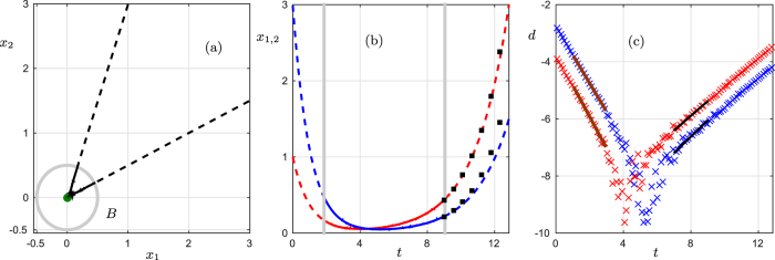
Figure 1. Dynamics near a planar saddle with small noise.

(a) Phase space (x₁, x₂) with a trajectory (black) passing near the saddle point. The stationary state (dark green dot) and a circle (gray) of radius r = 0.5 indicate a neighborhood of the stationary state outside of which the trajectory is shown as a dashed curve. (b) Time series for x₁ (red) and x₂ (blue). The gray vertical lines indicate entry and exit to the ball . The black squares are predicted values from the warning signals obtained inside B. (c) Plot of the logarithmic distance reduction d(T) as crosses; (see Supplementary Information, Section 2). The red/blue linear interpolants yield two approximations for the stable eigenvalue λ_s ≈ −1.10, −0.99 and the black lines for the important unstable eigenvalue λ_u ≈ 0.51, 0.57; the true values are (λ_s, λ_u) = (−1, 0.5). The black squares in (b) can be obtained from . Note that the choice of B is a choice of sliding window length (or lead time) for prediction as in the case for bifurcation-induced tipping.