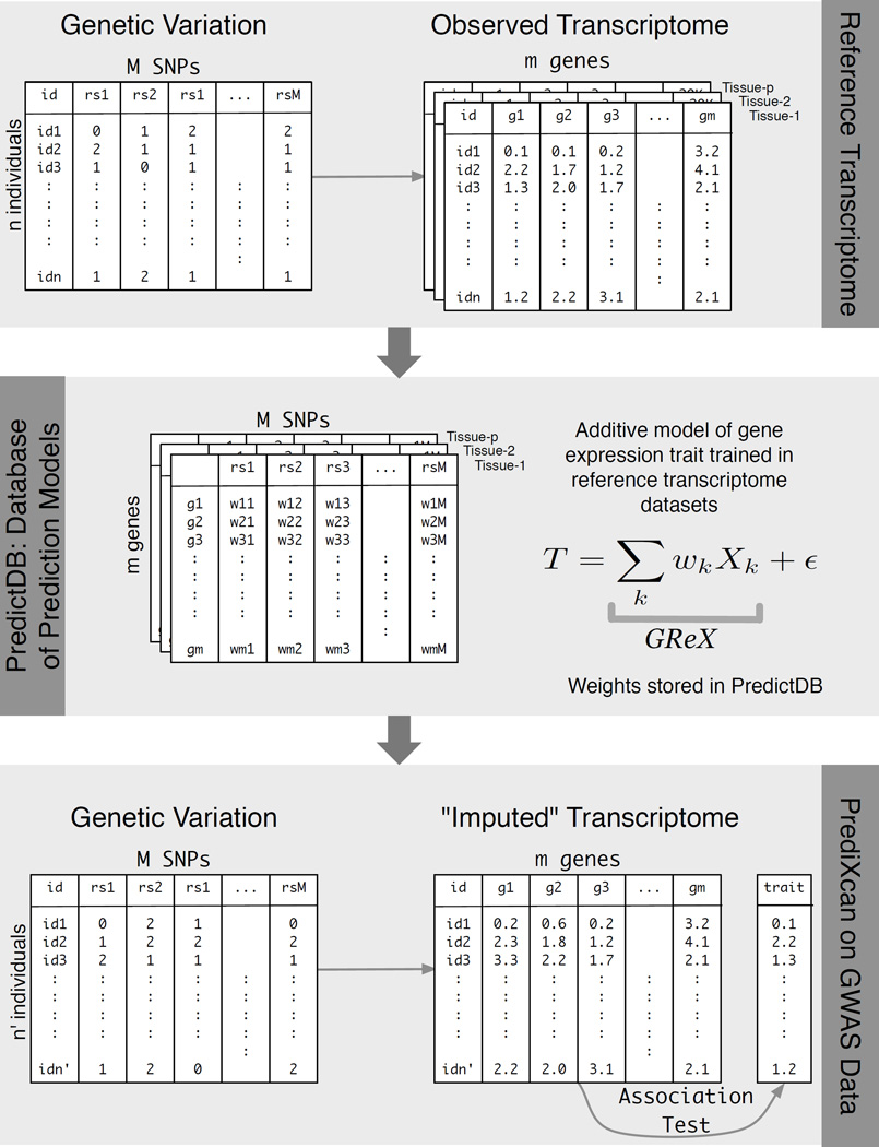
Figure 2. PrediXcan framework.
The workflow illustrates the steps used in developing the PrediXcan method. The top panel shows the data used from the reference transcriptome studies: genotype and expression levels (GTEx, GEUVADIS, DGN, etc). The sample size of the study is denoted by n, m is the number of genes considered, M is the total number of SNPs, and p is the number of available tissues. The second panel shows the additive model used to build a database of prediction models, PredictDB. T represents the expression trait, and Xk is the number of reference alleles for SNP k. The coefficients of the models for each tissue are fitted using the reference transcriptome datasets and optimal statistical learning methods chosen among LASSO, Elastic Net, OmicKriging, etc. The bottom panel shows the application of PrediXcan to a GWAS dataset. Using genetic variation data from the GWAS and weights in PredictDB, we “impute” expression levels for the whole transcriptome. These imputed levels are correlated with the trait using regression (e.g., linear, logistic, Cox) or non-parametric (Spearman) approaches. (For the disease phenotypes in the WTCCC datasets and the replication dataset reported here, we used logistic regression with disease status.)

