Fig. 3.

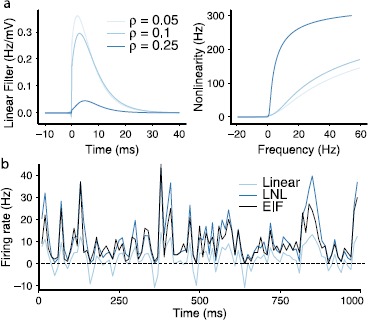
(a) The linear filter $A(t)$ and static nonlinearity F computed for inputs that yield several values of the spike correlation coefficient ρ. The filter receives a noise amplitude of $\sigma \sqrt{1-\lambda }$. The static nonlinearity receives a noise amplitude of σ. (b) The static nonlinearity applied to the linear estimate of the firing rate, for $\mu =0.1$, $\rho =0.1$, plotted over a randomly chosen 1000 ms time interval. The nonlinearity increases the firing rate magnitude and rectifies negative firing rates. This gives the predicted firing rates shown in blue; comparing with firing rates computed by binning spikes in 10 ms windows from simulations of the EIF model, shown in black, shows that the LNL is a fairly accurate model of the EIF dynamics