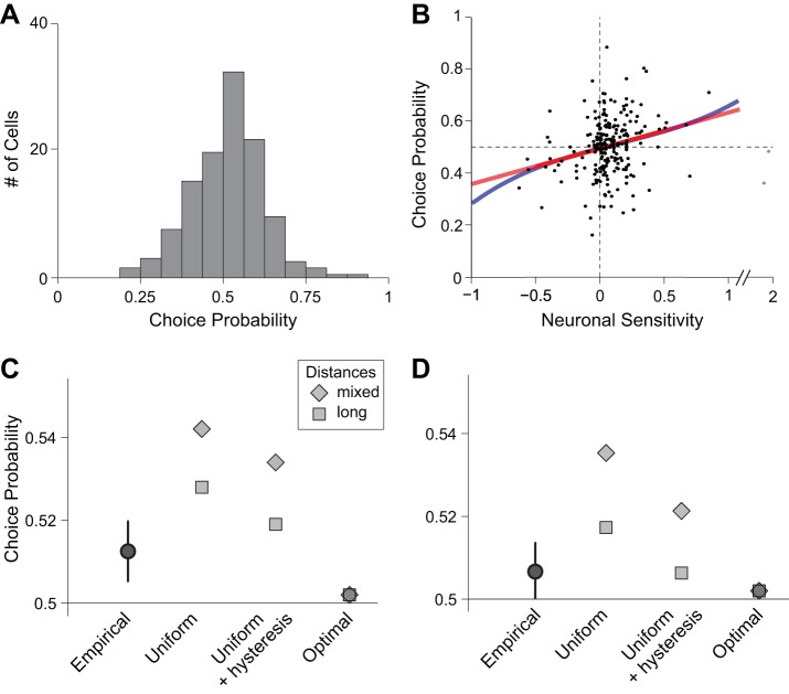
Fig. 7.

Choice probabilities and noise correlations. A: empirical distribution of CPs measured in the 500 ms after offer onset (N = 229 cells). Cells with positive and negative encoding were pooled (see materials and methods). Across the population, mean(CP) = 0.513 ± 0.007 (SE). B: relation between CP and neuronal sensitivity. Each data point represents one offer value cell. For each neuron, the neuronal sensitivity was calculated dividing the tuning slope by the average SD. Cells encoding the two juices (A and B) were pooled, but cells with negative encoding were not rectified here (sensitivity < 0). Color lines indicate the result of a linear fit (a₀ + a₁x; red line) and the result of a fit based on a third-order polynomial (a₀ + a₁x + a₂x² + a₃x³; blue line). In the latter, terms a₀ and a₁ were significantly >0, while terms a₂ and a₃ were indistinguishable from 0, indicating that the readout of offer value cells was close to optimal (Haefner et al. 2013). Two outliers (gray dots) were not included in the regressions, but adding them to the dataset did not alter any of the significance results. C and D: reconstructing choice probabilities from noise correlations. Each data point represents the mean(CP) obtained empirically or from a simulation (see results). The error bars shown for the empirical measure indicate SE. For each readout scheme, long-distance and mixed-distance simulations provided, respectively, a lower bound and an upper bound for mean(CP) (see materials and methods). Empirical and simulated CP were calculated during the postoffer time window (C) and the window 150–400 ms following offer onset (D).