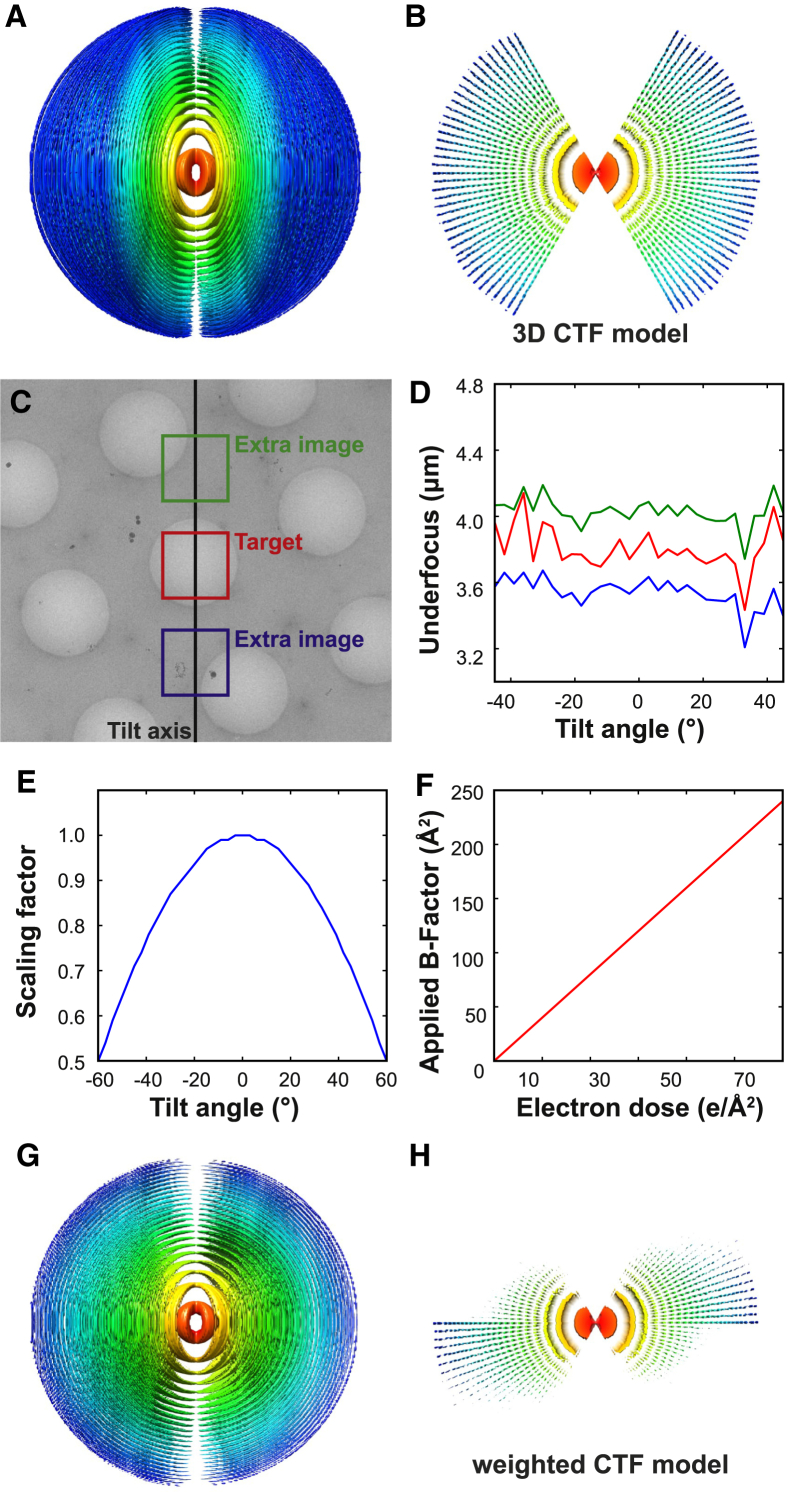
Figure 1.

3D CTF Model and CTF Estimation

(A) An isosurface view of the 3D CTF model used. The volume has been pseudo-colored based on radius (or resolution in Fourier space). Red indicates low resolution while blue indicates high resolution. The 3D CTF model is made of a series of 2D slices that represent 2D CTFs of each image of the tilt series.

(B) An orthogonal view of (A) with only the central slice shown.

(C) A low-magnification micrograph showing the extended tilt series acquisition used in this study. Two additional images were acquired to estimate the CTF parameters in the target region of interest.

(D) A plot of estimated defoci in each of the three regions shown in (C) at different tilt angles. The difference between the green and the blue curves might be caused by an inclination of the sample with respect to the tilt axis.

The diameter of holes in the micrograph is 2 µm.

(E) Tilt angle-dependent scaling factor applied to weight the 3D CTF model. The multiplicative factor is equal to the cosine of the tilt angle, and scales the entire CTF curve downward.

(F) Dose-dependent B–factor applied to the CTF model. The slope of the linear curve was determined empirically from a previous single-particle analysis report (Scheres, 2014).

(G and H) Isosurface view (G) and central slice (H) of the final weighted 3D CTF model.