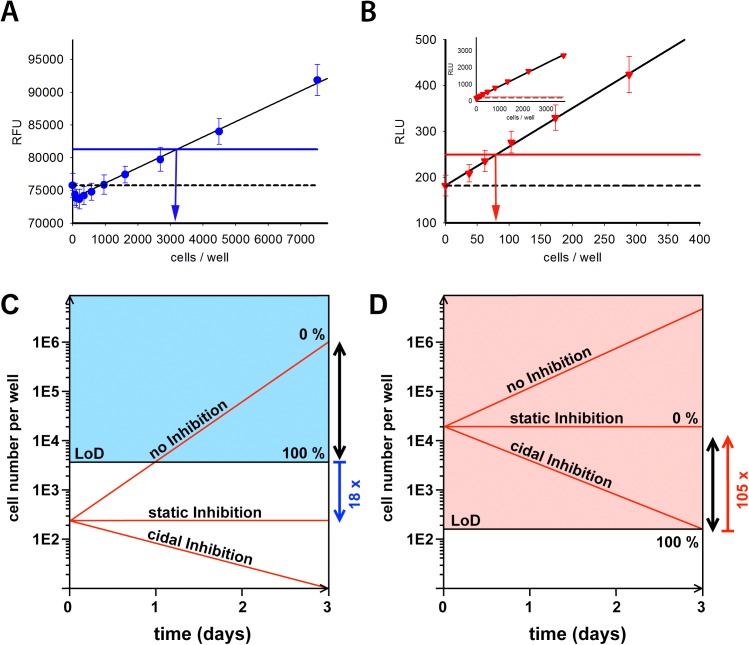
Fig 1. Limit-of-detection of historic and novel axenic assay and assay models.
A: Detection limit of the historic axenic assay. Black line shows the linear regression (R2 = 0.983, p < 0.0001). Dashed line shows average value of blanks. Blue line shows detection limit (3x standard deviation above the blanks value) for this assay. Vertical blue arrow indicates the number of cells at the limit of detection in this single experiment. Data is from a representative experiment of 4 with a minimum of 24 technical replicates. B: Detection limit of the novel axenic assay. Black line shows the linear regression (R2 = 0.998, p < 0.0001). Dashed line shows average value of blanks. Red line shows detection limit for this assay (3x standard deviation above the blanks value). Red vertical arrow indicates the number of cells at the limit of detection in this single experiment. Data is from a representative experiment of 4 with a minimum of 24 technical replicates. Inset shows data from a similar range of cell densities as used in 1A. C and D: The coloured areas represent cell densities that can be detected with the respective assay formats (C: historic axenic assay, D: novel axenic assay). Red lines represent different cell-growth inhibition scenarios during the course of this assay: compounds that do not inhibit cell growth (marked “no Inhibition”), compounds that arrest cell growth, without killing cells (marked “static Inhibition”), and compounds that kill cells (marked with “cidal Inhibition”). The black double arrows represent the analysis window. Blue (historic assay) and red (novel assay) arrows show the fold difference between the starting density and detection limit.

