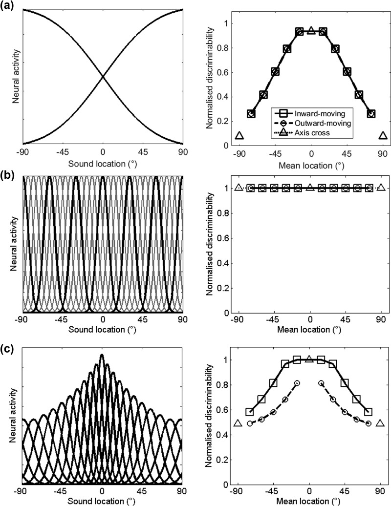
FIG. 2.

Models of sound location coding: The left-hand column shows representations of the models in terms of neural activity that would be expected for a given sound source location. The two-channel model (a) is represented by two Gaussians with means of −90° and 90° and standard deviation of 46°. The topographic model (b) is represented by multiple Gaussian curves located 6° apart with a standard deviation of 6. The modified topographic model (c) is represented by multiple Gaussian curves, with the midline represented by more and more narrowly tuned channels, the narrowest being 6° and the broadest, 12°. In (b) the channels are shown in gray with every tenth channel in black for visualisation purposes. The right-hand column shows the normalised discriminability (where 0 is chance and 1 is maximum performance) of the direction of the stimulus at the mean stimulus location based on the models. The two-channel model (a) discriminability is calculated as the change in the ratio of activity of each channel between the reference and target stimuli. In topographic (b) and modified topographic (c) discriminability is estimated by calculating the difference in Euclidean distance between the peak population activity generated by the reference and target sounds.