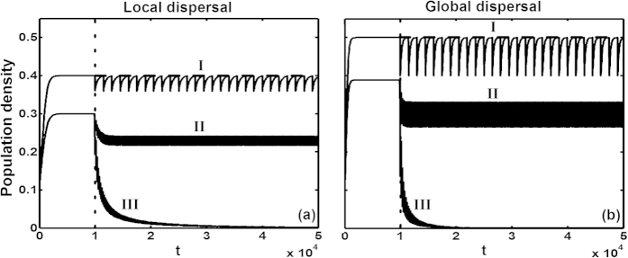
Figure 2. Three typical types of dynamic population behavior (see description in Methods) following spatially correlated periodic disturbance after t > 10000 (dotted line), regardless of dispersal traits.

Before disturbance (0 ≤ t ≤ 10000), the simulation was run until populations reached equilibrium density. Panel (a) with local dispersal: (I) species parameters (α, m, γ) = (0.01, 0.005, 0) and disturbance parameters (ρd, qd/d, T) = (0.1, 0.1, 1500); (II) (α, m, γ) = (0.01, 0.005, 0.002) and (ρd, qd/d, T) = (0.1, 0.1, 200); (III) (α, m, γ) = (0.01, 0.005, 0.002) and (ρd, qd/d, T) = (0.35, 0.35, 200). Panel (b) with global dispersal: (I) (β, m, γ) = (0.01, 0.005, 0) and (ρd, qd/d, T) = (0.2, 0.2, 1500); (II) (β, m, γ) = (0.01, 0.005, 0.003) and (ρd, qd/d, T) = (0.2, 0.2, 200); (III) (β, m, γ) = (0.01, 0.005, 0.003) and (ρd, qd/d, T) = (0.65, 0.65, 200).
