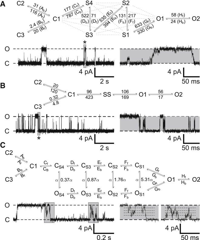
Figure 6.

Model simulations. (A) Model M1 after infrequent transition routes are excluded (M1-reduced). The model is adapted by adding two further closed states (C2, C3) and an extra open state (O2), to reflect the minimum number of closed and open time constants obtained from lifetime analysis. The number of Markov states for each individual subconductance state S1–S4 was kept constant at one. The model scheme is shown with only the transitions whose fitted rates were consistently larger than a threshold of 10⁻³ s⁻¹, across n = 8 voltage-dependent channels fitted at +30 mV. The all-to-all connectivity reduces to a linear scheme when connections that are not consistently frequent across all traces are discarded. Discarded connections are shown as gray dotted lines. These transitions did sometimes occur across the eight traces, but were not consistently present in all the channels (for example, see Table S4). Rates were obtained through a simultaneous global fit of the simplified linear scheme (M1-reduced) to eight channel recordings in QuB. These rates (s⁻¹) are given next to their corresponding connections, and are labeled A through H to correspond to the equivalently labeled rates shown in (C). An example of simulated openings is shown, and the asterisk indicates where an opening burst highlighted in gray is shown on an expanded timescale (right) to show typical features. (B) Model M2 after adaptation (M2-adapted) to include the same number of full open and closed states as the M1-reduced model (above). It was assumed that transitions O–C occur too infrequently to be included. Rates shown are from a simultaneous global fit in QuB to the data from eight voltage-dependent channels. An example of the model output is shown and the asterisk indicates where an opening burst highlighted in gray is shown on an expanded timescale (right) to show typical features. Time and current scales are equivalent to those in (A). The simulated traces exhibit superficial similarity to real recordings; however, the model produces a smooth range of subconductance amplitudes around a common mean unlike the subconductance events in experimental recordings. This is obvious in the amplitude histograms of the simulated data (black line) shown in Fig. S6. (C) Topology of a candidate fast gating scheme, which does not include any explicitly defined subconductance states and only contains fully open (O) or fully closed states (C). Rapid transitions between coupled pairs of closed and full open states labeled C_S4/O_S4, C_S3/O_S3, C_S2/O_S2, and C_S1/O_S1, result in observed subconductance state events of amplitude S4, S3, S2, and S1, respectively, after simulated events are low-pass filtered and resampled. Flickery gating arises from rates labeled α, where α is a fast rate (e.g., 50,000 s⁻¹). Transition rates between all remaining states are equivalent to those used in the M1-reduced model and are labeled A–H next to the transitions. A sample of the model output is shown with insets to the right showing subconductance gating on an expanded timescale. Again, amplitude histograms of the simulated data correspond well to experimental recordings (Fig. S7).