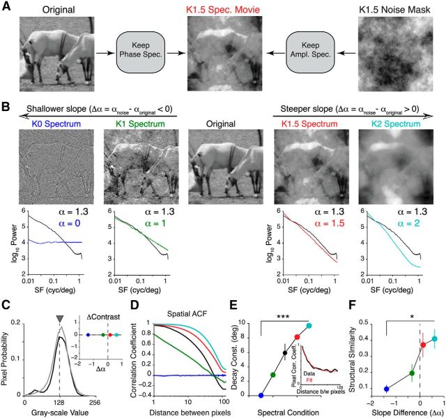
Figure 1.

Perturbing spatial correlations in natural movies. A, Illustration of the noise-masking procedure. Briefly, we combined the Fourier phase spectrum of a natural movie frame with the amplitude spectrum of a synthetic noise mask to create a noise-masked movie frame. B, Top, Example frames from a set of noise-masked movies with four different levels of spatial correlations. Bottom, Comparison between the power spectra of these movies (colored lines) and the original movie (black line). Note that the slope of all original movies used in this study is 1.3. C, Pixel intensity distribution from one original movie (black) and its noise-masked variants (gray). All noise-masked movies were adjusted to have the same luminance (gray triangle), contrast (see inset), kurtosis, and skewness as the original movie. Inset, A plot of the change in contrast against the difference in spectral slope, computed relative to the original movie. D, Representative spatial ACFs of the noise-masked movies shown in B. E, Spatial decay constant obtained by fitting a single exponential function to the ACF (inset). The decay constant decreased as spatial correlations were removed from the stimulus (p < 10⁻⁵, 5 movies). The inset shows that the ACF can be well fit with a single exponential function. F, SSIM between noise-masked movies and their original versions. The SSIM was averaged over frames for each movie (1200 frames in total). The p values for F and E were computed using the Cochran–Armitage test for trend. Error bars indicate SEM. Colors indicate noise-masked movies labeled in B. *p < 0.05; ***p < 10⁻⁴.