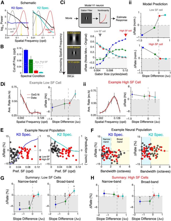
Figure 5.

SF tuning of neurons cannot explain responses to noise-masked movies. A, Schematic illustrating the portion of the power spectrum sampled by a typical low-SF- (gray) or high-SF-preferring (red) cell. The yellow arrow indicates the cutoff frequency, which is defined as the SF at which the power in the noise-masked movie is the same as that in the original movie. B, Quantification of the cutoff frequency (cycles per degree) for the different spectral conditions. As expected, cutoff frequency is the highest for K0 and lowest for K2 movies. Data are pooled from five movies. The gray lines show the mean ± SEM preferred SF of 308 neurons (four mice). Ci, Top, Schematic of an LN model of a V1 neuron used to predict responses to the noise movies. Briefly, a Gabor filter was convolved with a noise-masked movie, and the resultant was rectified with a pointwise nonlinearity to obtain a predicted firing rate. Bottom, Plot showing the predicted firing rate difference (ΔRate = noise movie rate − original movie rate) for Gabor filters of different sizes. Decreasing the size of the Gabor filter is equivalent to increasing the preferred spatial frequency. Cii, Plots showing predicted firing rate difference of a typical low-SF-preferring cell (top, SF denoted by gray arrow in Ci) and high-SF-preferring cell (bottom, red arrow). Di, Left, Representative tuning curve of a low-SF-preferring cell, which responds more to the spatially correlated movies. The SF tuning curve of this cell is well fit with a difference of Gaussians model (red line). Right, Plot of firing rate difference of this neuron demonstrating that this cell responds more to K2 movies. Dii, Same plot as Di, but for a high-SF-preferring cell that responds more to spatially decorrelated movies instead. E, Plots of the difference in firing rate against the preferred SF. Data are from 78 simultaneously recorded neurons. Dark gray dots indicate low-SF-preferring neurons (SF, <0.04 cpd), and red dots indicate high-SF-preferring neurons. Also plotted on the same axes is the difference in firing rate predicted from the model in C to illustrate the expected trend. There was no statistically significant trend in the data for either spectral condition (K0, p = 0.65; K2, p = 0.071; Spearman's rank correlation coefficient). F, Plots of the difference in firing rate against SF tuning bandwidth. The same neurons as in E were sorted according to bandwidth (see Materials and Methods). Similar to E, dark gray dots indicate low-SF-preferring neurons, and red dots indicate high-SF-preferring neurons. The dashed vertical line separates narrowband neurons (bandwidth, <2 octaves) from broadband neurons. G, H, Difference in firing rates plotted against difference in slopes for low-SF-preferring cells (G) and high-SF-preferring cells (H). Cells were further partitioned into narrowband and broadband based on tuning bandwidth. *p < 0.05; ***p < 10⁻⁴.