Figure 8.

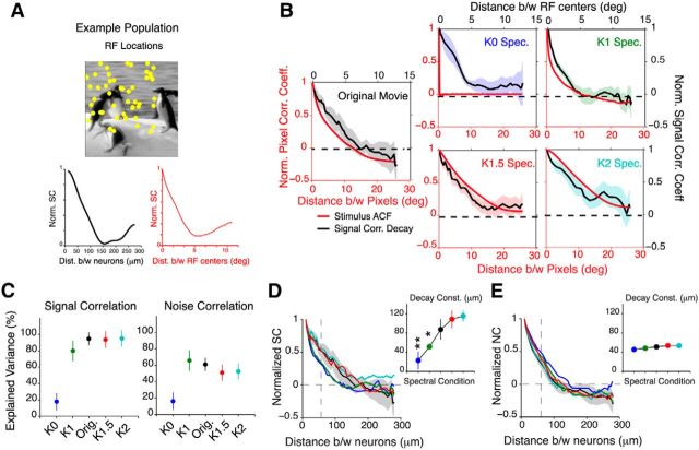
Spatial organization of interneuronal correlations closely tracks stimulus correlations. A, Top, Example RF locations of a population of 50 neurons. Note, the RF centers are not drawn to scale. Bottom, SCs between neurons in this example population decay with increasing distance between neurons (left) and increasing separation between RFs (Euclidean distance between centers, right). B, Comparison between signal correlation decay (black lines) and stimulus ACF (red lines) for all spectral conditions. The shaded area denotes the 95% CI of the median computed from 16 mice. In most conditions, the decay of signal correlations (except K0 movies) between neurons closely tracks the stimulus ACF. C, Explained variance of the fit between the stimulus ACF and the signal correlation decay function. The ACF is able to explain up to 80% of the decay in signal correlations and 60% of the decay in noise correlations. Data are presented as median ± 95% CI. D, E, Signal correlation (D) and noise correlation (E) as a function of distance between neurons for all spectral conditions. The inset shows the average decay constants estimated from single exponential fit. Data in the inset are shown as mean ± SEM. The shaded area in D indicates the 95% CI of the median of the original movie. All data in B–E are from 16 mice. *p < 0.05; **p < 10⁻³.