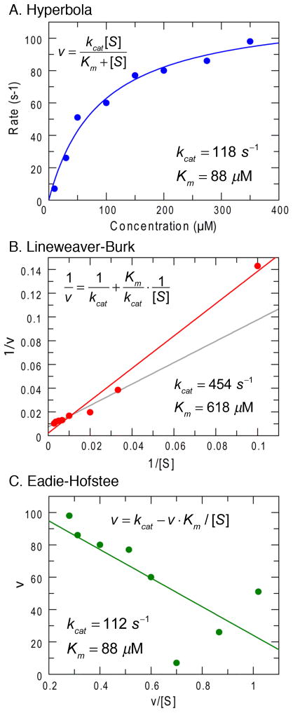
Figure 1. Comparison of three methods of fitting data to the Michaelis-Menten equation.
A. Data fit by nonlinear regression to a hyperbola. B. Data fit to a Lineweaver-Burk reciprocal plot. The gray line shows the fit obtained after omitting the point at the lowest substrate concentration. C. Data fit using the Eadie-Hofstee equation. In each figure, the equation and the resulting kcat and Km values are displayed.

