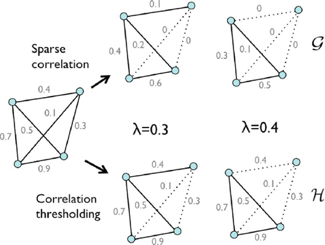
Fig. 2.
Comparison between the sparse correlation estimation via numerical optimization (top) and the proposed soft-thresholding method in Theorem 3 (bottom). The direct numerical optimization makes the graph sparse by shrinking the edge weights to zero. Nonzero edges form binary graph 𝒢. The persistent homological approach thresholds the sample correlations at given filtration value and construct binary graph ℋ. The both methods produce the identical binary graphs, i.e., 𝒢 = ℋ. If the methods are applied at two different parameters λ = 0.3, 0.4, we obtain nested binary graphs 𝒢(0.3) ⊃ 𝒢(0.4) and ℋ(0.3) ⊃ ℋ(0.4). Theorem 3 generalizes this example.

