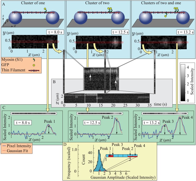
Fig 2. Cartoons describing the experiments and data analysis of Desai et al. [52].
A. Experimental set up and raw images for three different conditions: 1. (left) a single myosin bound to the thin filament; 2. (middle) two nearby myosin molecules bound to the thin filament; and 3. (right) three myosin molecules bound to the thin filament, two of which are close together. (Top) A thin filament is suspended between two silica beads (purple spheres) on a glass surface (gray). Variable concentrations of myosin head domains (S1), labeled with a fluorescent tag (GFP), are added to a solution that also contains variable concentrations of ATP and calcium. (Bottom) A camera records the fluorescence. Bound GFP-tagged S1s (GFP-S1s) appear as diffraction limited spots. In each simulated image, single GFP-S1s make a faint spot, while two nearby GFP-S1s make a brighter spot. The red box indicates the position of the thin filament. B. Construction of a kymograph. For each frame of a recorded movie, the pixels along the thin filament are isolated and stacked together, in chronological order, to make a 2-dimensional image. When GFP-S1s bind to the thin filament (inset, white arrows), they either increase the intensity of an existing spot if they bind near a bound GFP-S1 (left arrow), or they create a new spot (right arrow). C. Fitting the data with Gaussians. For a frame of a recorded movie, the pixels along the thin filament are isolated (top), and fluorescence is plotted as a function of position (bottom). Custom code [52] is used to fit these plots with Gaussians of constant standard deviation, but variable amplitude. Fluorescent intensity as a function of position, and the best-fit Gaussian(s), are shown for each of the different conditions in (A). Two nearby bound GFP-S1s (Peaks 2 and 4) are fit by a Gaussian with roughly twice the amplitude of the single bound GFP-S1 (Peaks 1 and 3). D. Construction of a histogram. For an entire movie, the amplitudes of the best-fit Gaussians of each individual frame are displayed as a histogram. The individual frames shown in (C) generate four amplitudes (red). The histogram is scaled so that the peak has an amplitude of 1. Note: scaled intensity, defined in the text, gives a single GFP-S1 an intensity of 1.

