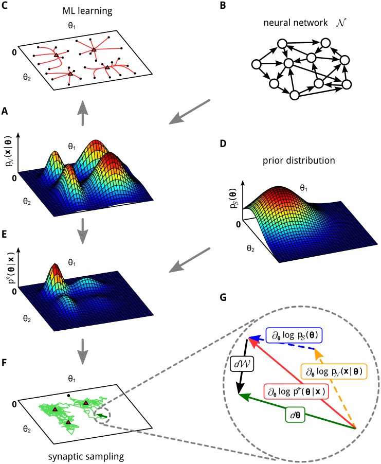
Fig 1. Maximum likelihood (ML) learning vs. synaptic sampling.

A, B, C: Illustration of ML learning for two parameters θ = (θ ₁,θ ₂) of a neural network 𝒩. A: 3D plot of an example likelihood function. For a fixed set of inputs x it assigns a probability density (amplitude on z-axis) to each parameter setting θ. B: This likelihood function is defined by some underlying neural network 𝒩. C: Multiple trajectories along the gradient of the likelihood function in (A). The parameters are initialized at random initial values (black dots) and then follow the gradient to a local maximum (red triangles). D: Example for a prior that prefers small values for θ. E: The posterior that results as product of the prior (D) and the likelihood (A). F: A single trajectory of synaptic sampling from the posterior (E), starting at the black dot. The parameter vector θ fluctuates between different solutions, the visited values cluster near local optima (red triangles). G: Cartoon illustrating the dynamic forces (plasticity rule Eq (3)) that enable the network to sample from the posterior distribution p*(θ∣x) in (E). Magnification of one synaptic sampling step dθ of the trajectory in (F) (green). The three forces acting on θ: the deterministic drift term (red) is directed to the next local maximum (red triangle), it consists of the first two terms in Eq (3); the stochastic diffusion term d𝒲 (black) has a random direction. See S2 Text for figure details.