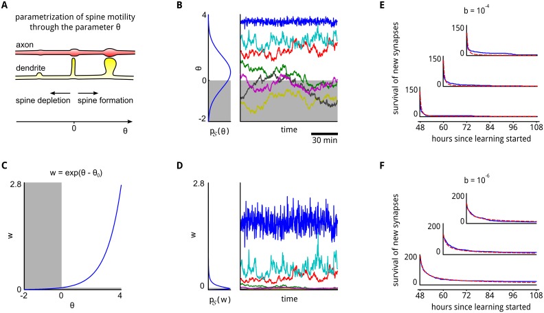
Fig 3. Integration of spine motility into the synaptic sampling model.

A: Illustration of the parametrization of spine motility. Values θ > 0 indicate a functional synaptic connection. B: A Gaussian prior p _𝒮(θ), and a few stochastic sample trajectories of θ according to the synaptic sampling rule Eq (10). Negative values of θ (gray area) are interpreted as non-functional connections. Some stable synaptic connections emerge (traces in the upper half), whereas other synaptic connections come and go (traces in lower half). All traces, as well as survival statistics shown in (E, F), are taken from the network simulation described in detail in the next section and S5 Text. C: The exponential function maps synapse parameters θ to synaptic efficacies w. Negative values of θ, corresponding to (retracted) spines are mapped to a tiny region close to zero in the w-space. D: The Gaussian prior in the θ-space translates to a log-normal distribution in the w-space. The traces from (B) are shown in the right panel transformed into the w-space. Only persistent synaptic connections contribute substantial synaptic efficacies. E, F: The emergent survival statistics of newly formed synaptic connections, (i.e., formed during the preceding 12 hours) evaluated at three different start times throughout learning (blue traces, axes are aligned with start times of the analyses). The survival statistics exhibit in our synaptic sampling model a power-law behavior (red curves, see S5 Text). The time-scale (and exponent of the power-law) depends on the learning rate b in Eq (10), and can assume any value in our quite general model (shown is b = 10⁻⁴ in (E) and b = 10⁻⁶ in (F)).