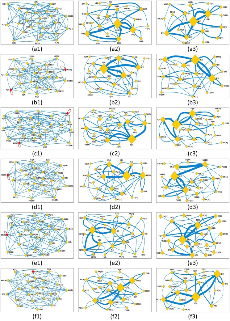
Fig 2. State transfer networks for fGms series.

Segment length is selected to be s = 5. Subplots (a1)-(f1) are the original state transfer networks for the fGm series with H = 0.5, 0.6, 0.65, 0.7, 0.75, and 0.8, respectively. The nodes that have self-links are marked with red color. The label x(y) means the state occurs for the first time at the position x along the time series (the x’th segment), and its identifier number is y; (a2)-(f2) The strong state transfer networks constructed by filtering out weak links (less than 25) in the original state transfer networks; (a3)-(f3) Shuffled networks. One can shuffle each original fGm series, and construct from the resulting series a shuffled network. Each displayed shuffled network is an average over 1000 realizations. Weak links also are filtered out. Except in the networks shown in (a1)-(f1), the size of a node indicates the occurring degree of the state. The width of an edge is the link’s weight.