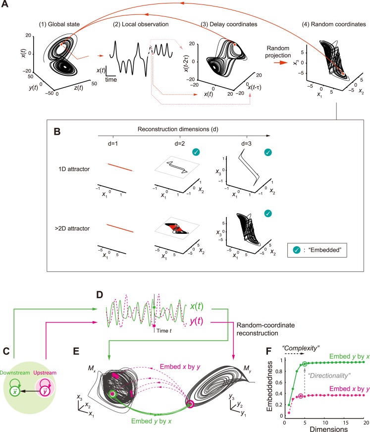
Fig 1. Cross-embedding analysis of complex network dynamics based on state-space reconstruction.

(A) Example of randomized delay-coordinate reconstruction assuming we observe dynamics determined with three-dimensional differential equation. (1) Global state is embedded using (2) temporal sequence of single observable of system. Attractor topology in global state space is fully recovered in (3) delay-coordinate of single observable. This relationship is maintained after (4) random linear projection of delay-coordinate space. Thus, there exists unique one-to-one map from (4) to (1), given sufficient number of coordinates. (B) The reconstruction needs sufficient dimensionality. Whether we have embedding or not depends on the relation between the reconstruction dimension (d) and the underlying attractor dimension (d _A). For example, a two-dimensional delay-coordinate space generically embeds one-dimensional attractor (e.g., a limit cycle, top row), except for a finite number of points. Higher dimensionality is required to embed more complex dynamics (bottom row). Generally, a dimensionality larger than that of an attractor (d > d _A) is necessary and sufficient for the embedding—to distinguish almost all states of the system [16] although perfect embedding without no self-intersection requires d > 2d _A [15]; the current cross-embedding protocol utilizes the former property. The Figure explores 1, 2 or 3 embedding dimensions after randomly projecting original delay-coordinates. Red regions indicate self-intersection with unignorable volume, reflecting incomplete embedding. (C) Unidirectional interaction between two modeled systems (directionally coupled Rössler systems, see Materials and Methods for equations). Downstream has information for whole system (light green) whereas upstream only has information on itself (light magenta). (D) Example of observed upstream and downstream signals. (E) The cross-embedding based on the random-coordinate state-space reconstructions. M _x and M _y respectively represent the downstream (x) and upstream (y) attractors based on single observed variable from each system. Colored arrows depict how nearby states in one attractor (disk: 20 nearest-neighbor states) are mapped onto states (dots) in other attractor (green: from x to y and magenta: from y to x). (F) Relationship between coordinate dimensions (number of randomized coordinates used for attractor reconstruction) and embeddedness (how accurately one node’s history can predict another node’s state). The circled dots represent complexity estimates, which were determined as minimum embedding dimension that provided ≥ 95% of optimal embeddedness measure (correlation between actual and forecast signals. See Materials and Methods).