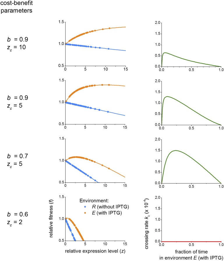
Fig. S8.

Robustness of landscape crossing for nonlinear cost–benefit tradeoffs. (Left) b and z_c are cost–benefit parameters used to convert relative expression levels into relative fitness (see Eq. S10 and Eq. S11). (Center) Relative fitness in each environment as a function of the measured average relative expression level for each genotype and for the b and z_c values on the left. Dots indicate experimentally measured average relative expression levels, and lines indicate Eqs. S10 and S11 plotted as a guide for the eyes. (Right) Crossing rate k_c in a variable environment scenario computed as previously described (environment dwell time $c=1/k_f=1$) using the relative fitness values from the corresponding figure in the center to compute the transition probabilities. Except for extreme cases (row 4; b = 0.6, z_c = 2), landscape crossing remains possible for moderate to strong nonlinear cost–benefit (rows 1–3). Rows 2 (b = 0.9, z_c = 5) and 3 (b = 0.7, z_c = 5) are qualitatively most similar to measured laboratory conditions of the WT lac operon (41).