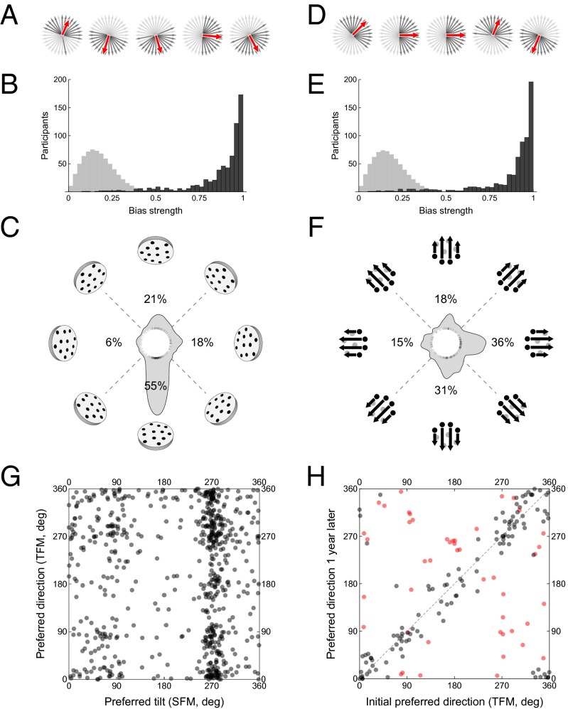
Fig. 2.

Results of the population distribution experiment (experiment 1). (A) Data of five representative participants (out of 691—the rest are shown in SI Appendix, Fig. S1) in the SFM condition. Data are represented using the conventions in Fig. 1 E and F. The red arrows are the bias vectors (Fig. 1 G and H). For visual clarity, only one out of four of the trials is shown. (B) Population distribution of bias strength (dark bars) compared with the null hypothesis arising from isotropically random tilt choice (light bars). Of the participants, 97.4% had significantly fan-shaped distributions (Rayleigh test, Benjamini–Hochberg correction for multiple tests with false discovery rate, 0.05). (C) Circular histogram of the population distribution of bias directions (smoothed using a 15 degree-wide kernel). Individual bias directions are shown as strokes on the rim of the white circle. Some corresponding plane orientations are shown for reference. The distribution is highly anisotropic (Kuiper’s test, P < 0.0001). Percentages indicate fractions of the population with peaks within ±45 degrees of the cardinal directions. (D–F) Corresponding results for the TFM condition, where 95.9% of observers had significantly fan-shaped distributions. The population distribution (E) resembles the distribution in a previous study (31), obtained with a much smaller sample in laboratory conditions. (G) Relationship between SFM and TFM bias directions, with each dot representing one participant. The two state variables are uncorrelated and independent. (H) Significant correlation between preferred TFM preferred directions as measured initially (x axis) and 1 y later (y axis), with each dot representing one participant. Participants whose preferred directions underwent significant change are shown in red. Similar results were obtained for the SFM preferred tilts.