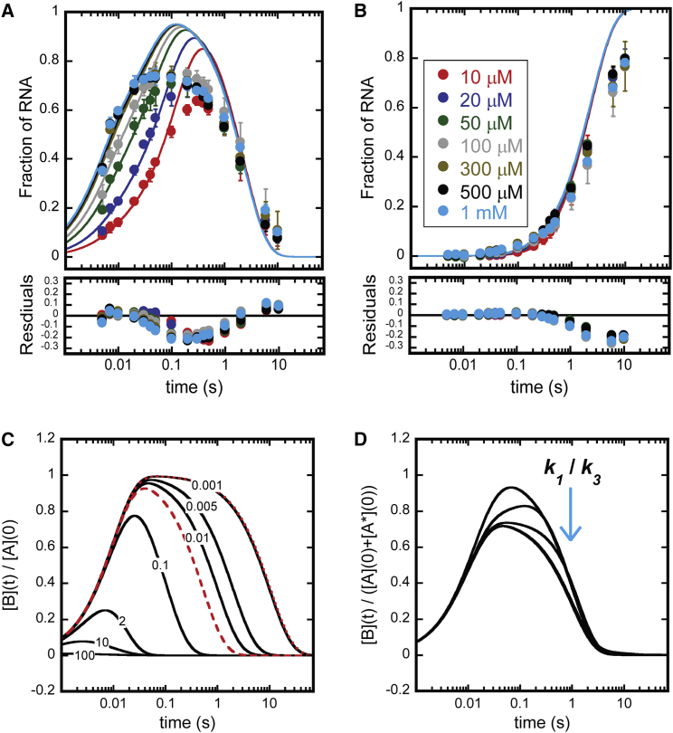
Figure 6.
Global fit of Scheme 1. Simulations of Eqs. 2 and 4. (A) Global WNLLS fit of 11-mer time course to Scheme 1. (Circles) Experimental data as described in Fig. 3A. (Solid lines) Scheme 1 simulated at best-fit parameter values. k1 = 1 × 10⁸ s−1, k2 = 5534 s−1, k3 = 142.8 s−1, k4 = 84.6 s−1, k5 = 52.3 s−1, and k6 = 0.43 s−1. (B) Global WNLLS fit of CA time courses to Scheme 1. (Circles) Experimental data as described in Fig. 3B. (Solid lines) Scheme 1 simulated at best-fit parameter values listed in the description in (A). (C) Evaluation of Eq. 2 at a range of k2/k1. Each trace is labeled with its respective k2/k1 ratio. For each evaluation, k1 = 100 s−1. To generate solid lines, k2 was set to the values {10,000, 1000, 200, 10, 1, 0.5, 0.1} s−1, to result in the k2/k1 ratio {100, 10, 2, 0.1, 0.01, 0.005, 0.001}, respectively. To generate broken and dashed red lines, k2 was set to the values {0.0955, 1.92} s−1 to result in the k1/k2 ratios {0.00096, 0.019}, respectively. (D) Evaluation of Eq. 4 at a range of k1/k3 ratios. For each evaluation, k2 = 100 s−1, k3 = 1 s−1, A(0) = 0.75, A∗(0) = 0.25. To generate solid lines, k1 was set to the values {50, 10, 2, 0.1, 0.01, 0.005, 0.001} s−1, to result in the k1/k3 ratios {50, 10, 2, 0.1, 0.01, 0.005, 0.001}, respectively. Note that below a k1/k3 ratio of 0.1, all curves overlay.

