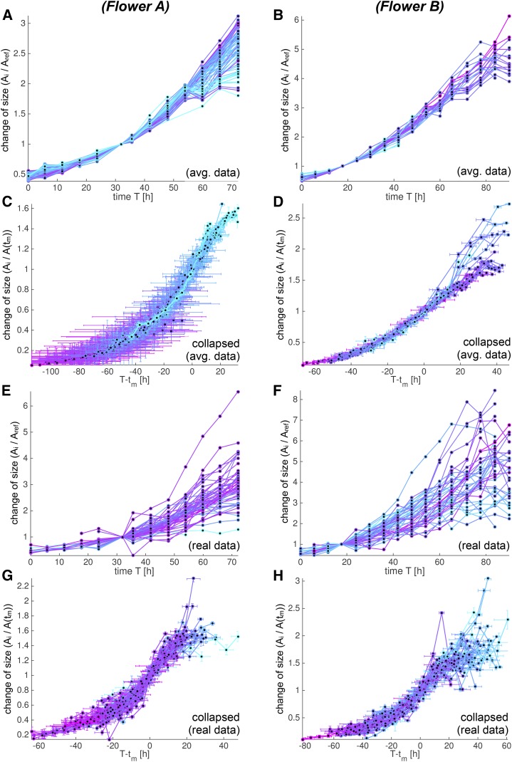
Figure 13.

Individual growth curves can be collapsed to similar S curves. We analyze growth curves for flowers A (A, C, E, and G) and B (B, D, F, and H) using both the spatially averaged (A–D) and the real (E–H) data. The growth curves are colored according to t_m (early [cyan] to late [purple]). A, B, E, and F, The individual growth curves f(T) show the change in each cell lineage area in time compared with the reference time. The curve f(T) is only defined at discrete time points T = t_i marked with dots [f(t_i) = A_i/A_ref]. We only consider data with a meaningful fit to an S curve. C, D, G, and H, We collapsed the growth curves into more similar curves by aligning them according to the nearly constant RGR(t_m). We aligned them in time by removing the dependency of t_m, and we scaled the curves according to their size at time t_m such that their slope corresponds to RGR(t_m). We therefore computed f_c(t) = f(t + t_m)/f(t_m) and plotted f_c(t) against t = T – t_m. Both t_m and f(t_m) were estimated from the best-fitting S curve, whereas we evaluated f(t + t_m) at discrete time points t = t_i – t_m from the actual data [f_c(t_i − t_m) = A_i/A(t_m)]. Note that since f still depends on three of the four parameters defining the S curve, it was not obvious the curves would collapse to a single curve. The fact that the transformed growth curves f_c(t) lined up well confirmed that the RGRs at times t_m and t_x were the same for each cell lineage.