Statistical relevance—relevant statistics, part I

Abstract

As part of a new EMBO Journal statistics series, this commentary introduces key concepts in statistical analysis and discusses best practices in study design.

Statistical analysis is an important tool in experimental research and is essential for the reliable interpretation of experimental results. It is essential that statistical design should be considered at the very beginning of a research project, not merely as an afterthought. For example if the sample size for an experiment only allows for an underpowered statistical analysis, then the interpretation of the experiment will have to be limited. An experiment cannot be reverse engineered to become more statically significant, although experiments can of course be repeated independently to account for biological variation (see section on technical versus biological replicates below). Statistical methods are tools applied to situations in which we encounter variability, noise and uncertainty. They help make more definitive scientific conclusions, and to make better use of available resources.

In this new EMBO Journal statistics series, I will introduce key concepts and best practices. The text will be short and conceptual in style, while the supplement will provide examples demonstrating the introduced concepts. I will use the free statistic software R (R Core Team, 2015) to illustrate examples, and readers can try the code on their own data.

In this first part, I will give some guidelines for initial study design and analysis of experiments. Subsequent columns will discuss specific statistical topics in more detail. Most of the issues touched upon in this first column are further discussed in the book of Ruxton and Colegrave (Ruxton & Colegrave, 2010), which includes many examples relevant to the analysis of experiments for biological researchers.

Guidelines and terms for the design and analysis of experiments

Experiment versus study

The terms experiment and study are sometimes used interchangeably, but they represent different concepts. In an experiment, one uses highly controlled conditions to look at a (model) system, performs specific well‐designed interventions at controlled times and intensities, and has an efficient assay to measure the effect of interest. You control the “experimental units” (such as cells, mice, and genotypes) and plan which experiments to perform and when. This allows for a stringent control over experimental variables and to draw very specific conclusions. However, this comes with the inherent risk of exerting too tight control—for example, the model system may not be relevant and therefore not support the hypothesis you are testing, or the controlled conditions might not be exactly the right ones.

On the other hand, the observations in a study are made “in the wild”—for example, on human subjects recruited to a study according to certain inclusion and exclusion criteria, but still taking into account their individual history, genetic makeup, and lifestyle. Likewise, an ecologist studying animals or plants encountered in the field does not have full control over their environment or other potentially important variables. Generally, a study requires much bigger sample size than an experiment and is more complicated to analyze, usually requiring involvement of a specially trained expert at some point. In this series, I will mainly focus on the analysis of experiments.

Hypothesis‐driven research

Although there are various “hypothesis‐free” exploratory experiments, such as the sequencing of a genome or the genome‐wide binding site mapping of a transcription factor, it is important to remember that most biological experiments are hypothesis‐driven. This means that an experiment should be based on a scientific question or hypothesis—although this may sound obvious, it is a point that is sometimes neglected.

As a general rule, do not plan your experiments as an accumulation of conditions (e.g. “Do cells treated with drug A for 20 or 40 min express protein X but not Y?”)—instead start with clear, single research questions, one at a time like:

• Is drug A better than drug B in inducing a given effect?

• Is there a genetic interaction between gene X and gene Y?

• Are transfected cells behaving differently than control cells?

Only then should one consider important choices such as which model, which conditions, which intervention, or which readout to use?

Controls & replicates

Imagine you want to use proteomics to study the effect of different doses of a cytokine on the phosphorylation of cellular downstream targets over time. Further assume that the cells used are inexpensive and easy to culture, but the proteomic analysis is expensive and time‐consuming. In this scenario, there is a tradeoff between the number of conditions and the temporal resolution you can achieve. Importantly, the expected effect size should guide the design of the experiment: The higher the expected effect, the lower the number of biological replicates that are needed—in this example, to reliably detect protein phosphorylation. If the cytokine is known to affect its target proteins fairly quickly, then only a few time points and few replicates per time point are needed. If, on the other hand, the expected differences between the conditions are more subtle, then more replicates per condition might be required. In cases where a high temporal resolution is achievable, this can serve as a legitimate internal control: A higher number of time points can make up for fewer replicates, since the measurements are related due to their temporal proximity.

Experimental units and control categories

The choice of experimental units is a subtle point. Very often, experimental units will simply be the biological units used, such as mice, yeast strains or cultured cells. However, experimental units can also be time periods, for example, if animals receive a specific treatment for defined periods of time—not the animal but rather the treatment time would be the experimental unit here.

Another important aspect when deciding on experimental units is the choice of appropriate controls. The two major categories are positive and negative controls: Positive controls show that an experimental system works in principle, while negative controls represent a baseline (e.g. wild type) condition.

For an example, let us assume we want to knock down, using short‐interfering (si) RNAs, the expression of certain genes to study their influence on intracellular protein transport. Here, a negative control could be sequence‐scrambled siRNA applied to the cells, while a positive control for the working of the assay system could be a siRNA against a gene with an already known role in intracellular transport. It is furthermore advisable to establish an “experimentalist control” by “blinding” the experimenter to ensure that s/he does not know which condition the readout belongs to.

For a thorough discussion of various different types of controls, see Glass (2014) (Section 3 therein).

Blocks/batches

We aim to perform experiments within a homogeneous group of experimental units. These homogeneous groups, referred to as blocks, help to reduce the variability between the units and increase the meaning of differences between conditions (as well as the power of statistics to detect them).

For example, it is beneficial to take measurements for many (ideally all) experimental conditions at the same time. If the measurements are done over a more extended period of time, then day‐to‐day variability between the measurements needs to be estimated and eliminated. If all control conditions are measured on one day and all treatment conditions on another day, then it is not possible to disentangle the day effect from the treatment effect and, in the worst case, the data become inconclusive. As a general rule, at least some “common conditions” are essential to assess potential block effects.

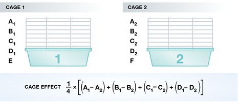
As an example, assume there are six treatment conditions you want to apply to mice (the experimental units), but you can fit only five mice per cage (i.e. block). In this case, not all treatments can be applied simultaneously in each cage/block. You can, however, apply four identical treatments to each of the cages and only alternate the fifth condition each time (see Fig 1). Now, the “cage effect” can be estimated by computing the mean of the differences between the four treatments that are identical, as given by the formula in Fig 1. A priori the conditions E and F are not directly comparable since they were measured on mice from two different cages. However, the replicated treatments allow a computation of a “cage effect” that corresponds to the average difference between the identical conditions measured in the two cages. Then, the difference between E and F can be computed as E − F − “cage effect”.

Figure 1. Example of a simple batch effect correction.

Illustration of batches and how to correct for them. All but two treatments have been applied to mice in two different cages (= batches). The batch/cage effect can now be computed based on the treatments that are shared between the cages.

Undiscovered block effects that strongly influence the result of the experiments are commonly called batch effects and they may cloud scientific conclusions. The severe influence of batch effects has been revealed in high‐throughput experiments (Leek et al, 2010); Importantly, batch effects also exist in small‐scale experiments, but are harder to detect, and while they may affect the scientific conclusions, they often remain hidden.

In practice, drafting a plan detailing which measurements to perform is very helpful in order to maximize the number of measurements within one batch, or to try to balance the conditions of interest within the batch. For data tables, it is a good idea to add as much useful metadata (e.g. date, time, and experimenter) as possible. As an example, see Table 1.

Table 1.

An example of a comprehensively annotated data table

Condition	Time	Target	MS run	Technician	Signal intensity
40 ng/ml HGF + AKTi	10 s	pMEK	5567	A	5579
40 ng/ml HGF + AKTi	20 s	pMEK	5567	B	3360
80 ng/ml HGF	10 s	pAKT	6650	A	8836

Randomization

Even after careful identification of blocks, other factors may still influence experimental outcome, such as mouse age and sex differences, and different genetic backgrounds. In order to balance out these factors, randomization techniques are used. Randomization reduces confounding effects by equalizing variables that influence experimental units and that have not been accounted for in the experimental design. This requires randomly allocating the experimental units to the experimental conditions. Thus, ideally, the allocation of units to conditions should not be predictable.

For example, if an experiment compares the effect of a genetic modification on tomato growth, many potentially complex factors apart from the genetic modification itself could influence growth: For example, the growth chamber could be slightly warmer on one end than the other, the quality of the compost variable, or different irrigation techniques used. In this case, it will be necessary to randomize the positioning of the plants.

Replication

Replication of measurements is very important. Without replication, it is impossible to judge whether there is an actual difference between conditions, or whether an observed difference is merely due to chance.

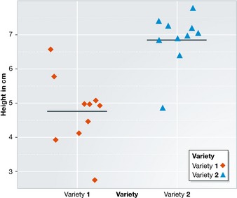
For example, if you would like to compare the height of two plant varieties by only taking one plant height measurement and observing a difference of 10 cm, it is impossible to say whether this difference is meaningful or due to natural variation. On the other hand, if multiple plants of each variety are measured, and the height differences always turn out somewhere around 10 cm, the observed difference is less likely due to chance, as illustrated in Fig 2. The difference is strong relative to the variability between the measurements.

Figure 2. A comparison between two groups.

Comparison of two groups. The difference is strong relative to the variability between the measurements within each group.

Technical versus biological replicates

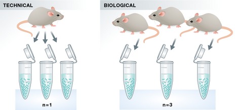
When referring to replicates, it is important to distinguish between biological and technical replicates (see Fig 3). Technical replicates refer to experimental samples isolated from one biological sample, for example preparing three sequencing libraries from RNA extracted from the cells of a single mouse; in contrast, biological replication would mean extracting RNA from three different mice for the comparisons of interest. In other words, it is not sufficient to merely “re‐pipet” an experiment from the same sample, as this does not constitute biological, but merely technical replication. In general, technical replicates tend to show less variability than biological replicates, thus potentially leading to false‐positive results. Technical replicates can be useful when a new technique is reported, but, in general, biological replicates should be reported. Either way, this has to be clearly labeled in a paper and technical and biological replicates should not be integrated into a single statistic.

Figure 3. Technical versus biological replicates.

Illustration of the difference between technical and biological replicates.

Outlook

After the experimental data have been obtained, a next step is to look at the data via exploratory graphics. Appropriate graphics are also very important for the final presentation of the work. In the next column, best practices for the display of both numerical and categorical data will be introduced and suitable estimators for the mean and the variance of the data will be discussed.

Conflict of interest

The author declares that he has no conflict of interest.

References

- Glass DJ (2014) Experimental Design for Biologists, 2nd edn Cold Spring Harbour, NY, USA: Cold Spring Harbor Laboratory Press; [Google Scholar]
- Leek JT, Scharpf RB, Bravo HC, Simcha D, Langmead B, Johnson WE, Geman D, Baggerly K , Irizarry RA (2010) Tackling the widespread and critical impact of batch effects in high‐throughput data. Nat Rev Genet 11: 733–739 [DOI] [PMC free article] [PubMed] [Google Scholar]
- R Core Team (2015) R: A Language and Environment for Statistical Computing. Vienna, Austria: R Foundation for Statistical Computing; [Google Scholar]
- Ruxton GD, Colegrave N (2010) Experimental Design for the Life Sciences, 3rd edn Oxford: Oxford University Press; [Google Scholar]