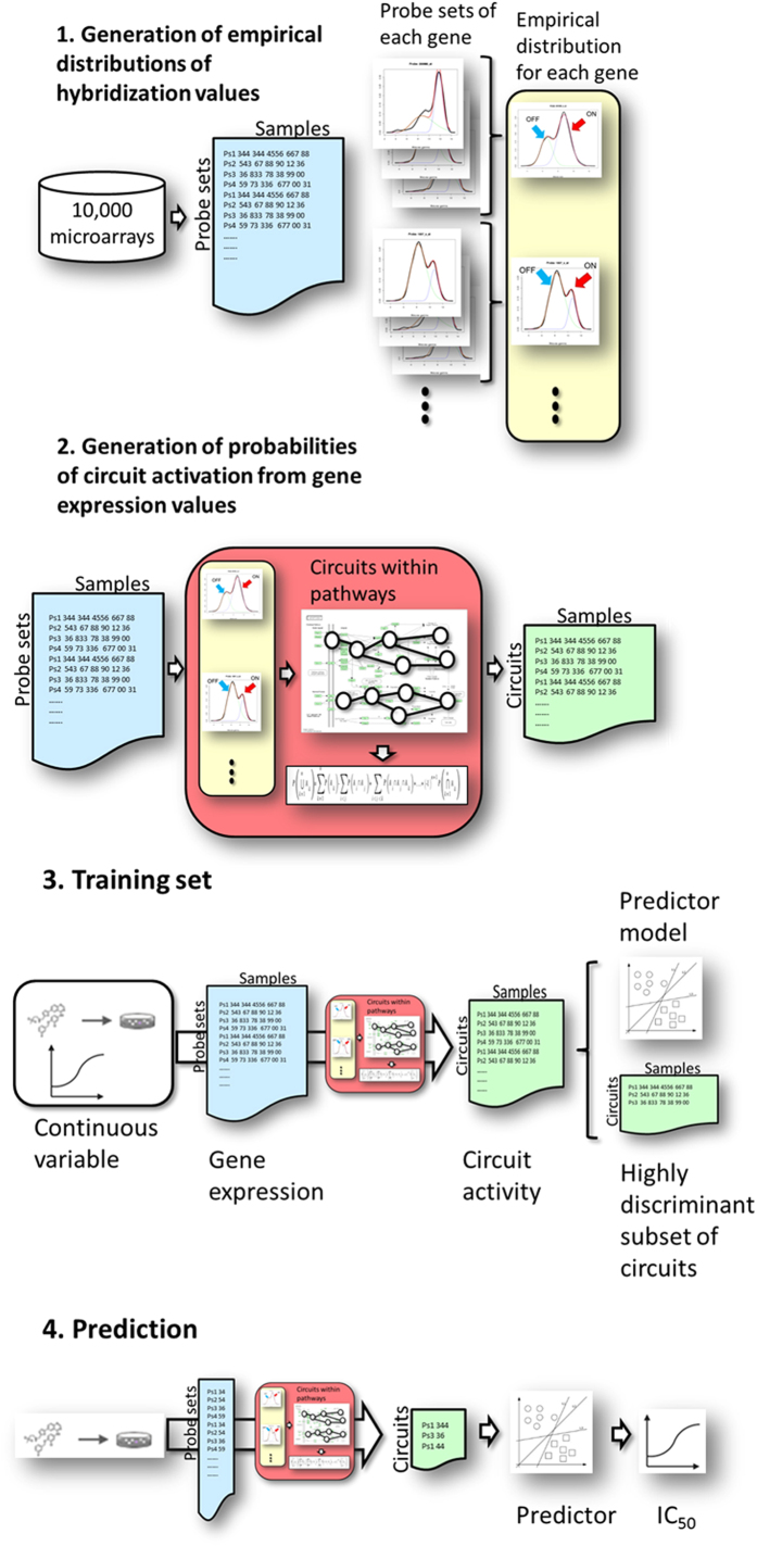
Figure 6. Steps for the generation and use of predictors based on signaling circuit activities.

Step 1: generation of the empirical distribution of probeset values. A collection of more than 10,000 microarrays representing an enormous diversity of conditions is collected from the GEO database. For any of the probesets, an empirical distribution is derived and a mixture model is used to define the highest value peak, which corresponds to an active probe (ON), and the lowest peak that correspond to the probeset (OFF). Gene values can be obtained by summarizing the corresponding probeset values. Step 2: Given one or several microarrays, the probeset values can be contrasted with the empirical distribution values to obtain the corresponding activity probabilities which are used to derive gene activity probabilities. These, within the context of the circuits defined, are used to estimate circuit activity probabilities. Step 3: an initial training set is required to derive obtain the predictor. Gene expression values from individuals from two classes, or from different treatments (dosage, time, etc.) are obtained and transformed (as described in step 2) into the corresponding profiles of signaling activities. Then, a feature selection method obtain a sub list of highly discriminative circuits which is used to train the predictor (see below). Step 4: once the predictor is trained it can be used to predict class membership for an unknown sample (or to predict a continuous value from gene expression measurements). Gene expression values from the sample are transformed into the corresponding pattern of signaling circuit activities (see step 2) of the sample. The predictor is then used to predict the class to which most likely the sample belongs to. Identically, gene expression values of a series of conditions can be used to predict the corresponding continuous value (not shown in the figure).