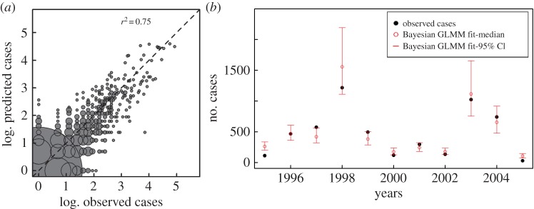
Figure 3.

Comparison of predictions and observations for the GLMM model that includes structured and unstructured random effects. In (a), kebele-season predictions are plotted against observations in the log scale, with the identity line in the diagonal (dotted line). Predictions are generated by sampling from the posterior distribution of fitted parameters 10 000 times for 159 × 11 kebeles-seasons and computing the median cases from the simulations. Because the number of prediction–observation pairs at a given point can be (much) higher than 1 (e.g. 963 at the origin), we represent this number by the size of each circle centred at that pair. (Size is specifically scaled by the square root of the frequency.) Thus, although some predictions depart from observations for the kebeles and seasons with no cases, the instances of these discrepancies are very few compared to the bulk of correct predictions. Similarly, for observed non-zero cases, the majority of the predictions fall along the diagonal. See the electronic supplementary material, figure S4, for a version of this graph that includes another representation of the uncertainty around predictions. In (b), predictions of JFMA cases are aggregated for all kebeles and shown in time for the different years. From the 10 000 parameter combinations, the medians of the aggregated cases for a given season are shown together with the 95% credible intervals (CI) (the 2.5% and 97.5% quantiles of the simulated JFMA cases). The GLMM 95% CI include the observed cases 64% of the time (and 82% of the predictions within 7% of the CI intervals).