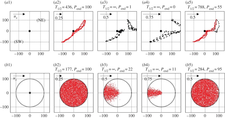
Figure 3.

Simulations of the IBM under different initial conditions. (a1) ‘Release’ set-up, illustrating release locations relative to the goal (central dot). (a2–a5) Representative tracks for (a2) u_x = 0.25, k = 1.0, (a3) u_x = 0.5, k = 1.0, (a4) u_x = 0.75, k = 1.0 and (a5) u_x = 0.5, k = 1.5. Successful (solid red lines) and unsuccessful (black dashed) tracks are differentiated. The direction and flow strength are indicated by the top left arrows, while measures P₁₀₀₀ and T_1/2 are given above each plot. (b1) ‘Uniform’ set-up with individuals distributed across the circular region surrounding the goal (central dot). (b2–b5) Initial locations of individuals that reach the goal by t = 1000 are marked by red dots for (b2) u_x = 0.25, k = 1.0, (b3) u_x = 0.5, k = 1.0, (b4) u_x = 0.75, k = 1.0 and (b5) u_x = 0.5, k = 1.5. Note that we only show the centre of the full region, where L_x = L_y = 300. (Online version in colour.)