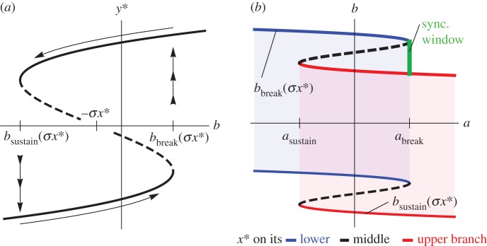
Figure 2.

Coupling a slave subsystem to a master subsystem moves the slave subsystem's tipping points and can change them suddenly. (a) The bifurcation diagram of the slave subsystem shows the equilibrium of the slave subsystem y*(b; σx*) as a function of its slow parameter b. (The slave subsystem's equilibrium y* also depends on the coupling term σx* due to the influence of the master subsystem.) In this example, the master subsystem has just passed its break point a > a_break, so the master subsystem has quickly moved to its upper stable branch of equilibria (x* > 0). Because the coupling strength σ > 0, the sudden shift in the master subsystem makes it easier for the slave subsystem to pass its break point [b_break(σx*) < b_break(0)]. (b) The locations of the saddle-node bifurcations of the slave subsystem (equation (2.2b)), denoted by b_break(σx*) and by b_sustain (σx*), are one- or three-valued functions of a, the parameter of the master subsystem. The colours match those in figure 1: if the master subsystem's equilibrium x* lies on its lower (respectively, upper) stable branch depicted in figure 1b, then the bifurcation points of the slave subsystem are the blue (respectively, red) curves in (b). There exist three equilibria y* in the shaded blue (respectively, red) regions. Here, σ > 0, so the master subsystem acts to prevent the slave subsystem from crossing its break point b_break(σx*) when x* < 0 and facilitates it when x* > 0. If (a,b) crosses the green line segment marked ‘sync. window', then the regime shifts synchronize: the master subsystem (equation (2.2a)) crosses its break point a_break, causing x* to jump from a negative number to a positive number, which causes the slave subsystem (equation (2.2b)) to cross its break point b_break(σx*).