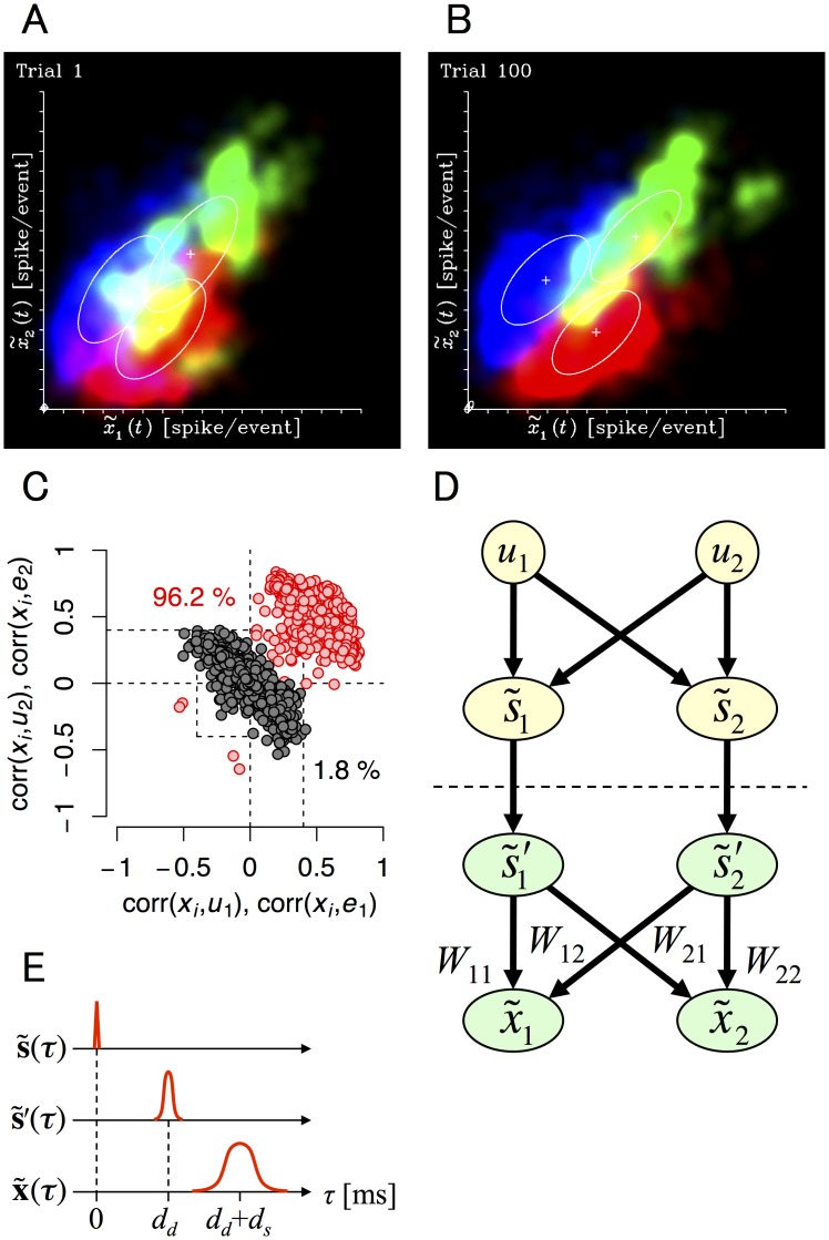
Fig 7. Population activity of cultured neural networks.
Absence of stimulus classification before learning (A) and its presence after (B); summary of classification statistics (C); summary of the inverse recognition model (D) and dynamics of the inverse recognition model (E). (A) Evoked responses of populations of cultured neurons before training. Horizontal and vertical axes are the averaged responses of u 1- and u 2-preferring electrodes ( and ). Red, blue, and green indicate evoked responses when the state of u is (1,0), (0,1), and (1,1), respectively. The Fig corresponds to a superimposition of responses at t = 1, …, 256 from 23 cultures. Plus-marks and ellipses are the means and standard deviations of given u averaged over 23 cultures. The scale indicates the averaged spike number per stimulation. (B) Evoked responses after training. The evoked response transient throughout training is shown in S3 Movie. (C) The distribution of correlation. Red circles plot the correlation of x i with u 1 (horizontal) and u 2 (vertical) (n = 1035 electrodes from 23 cultures). Black circles plot the correlation of x i with e 1 (horizontal) and e 2 (vertical), where e 1 and e 2 are the error of x i from u 1 and u 2, respectively. (D) Schematic image of a population model under the assumptions of the inverse recognition model. Our model assumes that is a column vector of inputs, ’ and are column vectors of the population activity of neuron groups, and W is a 2 × 2 matrix of connection strengths. Also, we assume that can be represented as a multiplication of the connection strength matrix W by ’ (linear, firing-rate neuron model). Based on the recognition model, W was calculated from the relationship between the amplitude of the stimulation and the evoked response using the maximum likelihood estimation. (E) Dynamics of the inverse recognition model. Upper, middle, and lower time courses represent input, direct response, and synaptic response, respectively.

