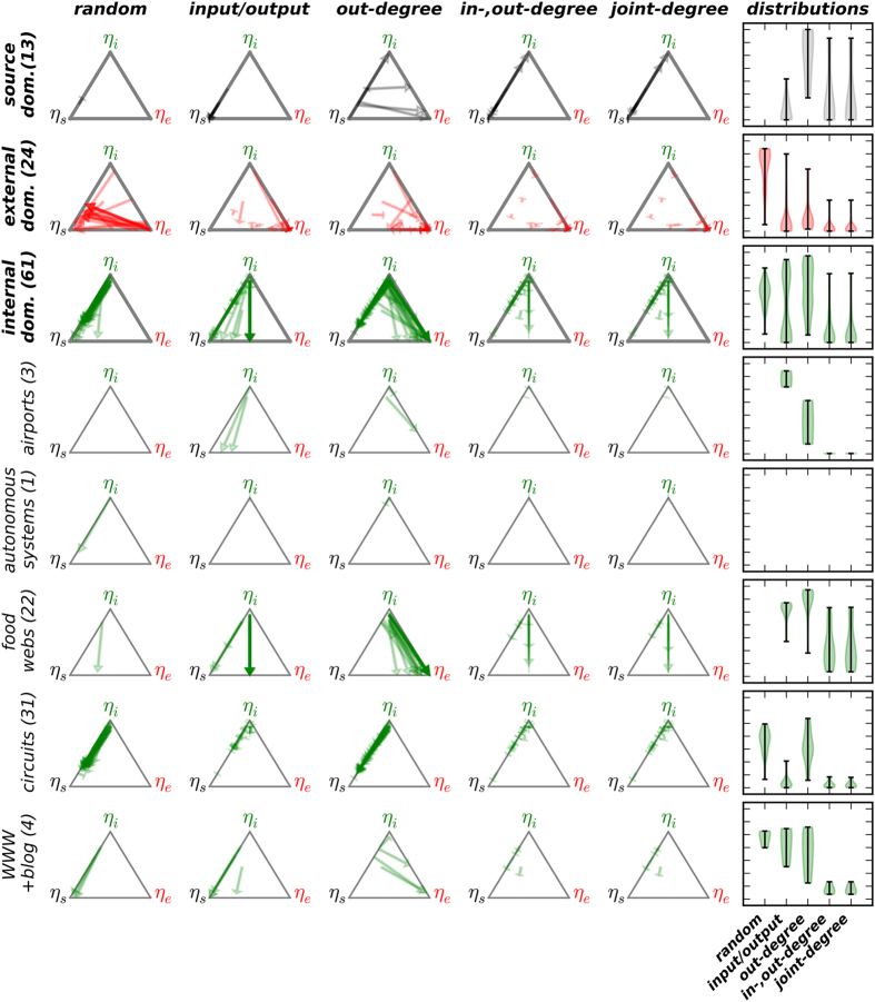
Figure 2. Behavior of the control profile of empirical networks under null models that preserve: (random) only the number of nodes and edges, (input/output) the number of source and sink nodes, (out-degree) the out-degree distribution and number of source and sink nodes, (in-,out-degree), both the in- and out-degree distributions, and (joint-degree) the joint-degree distribution.

A total of 98 networks are categorized as dominated by η_s, η_e, or η_i (top three rows, respectively shown with black, red, and green vectors); the η_i-dominated networks are further shown in five subcategories (bottom rows). In each panel, ternary plots show semi-transparent vectors pointing from the original control profile to the mean control profile over 10 randomizations (the low replication number is justified because the standard deviations are already very small at this point: mean <0.025, median <0.002). Vector tips are drawn with uniform width and length proportional to the overall length of the vector; as such, very short vectors are indicated with a thin line perpendicular to the orientation of the vector. Networks with a control profile = (0,0,0) are not shown¹³. The rightmost column shows the distribution of vector lengths (i.e., Cartesian distances) with a uniform vertical scale for each row, omitting plots with 0 or 1 vectors. The shorter the vector lengths, the better is the agreement between a null model and the empirical networks.