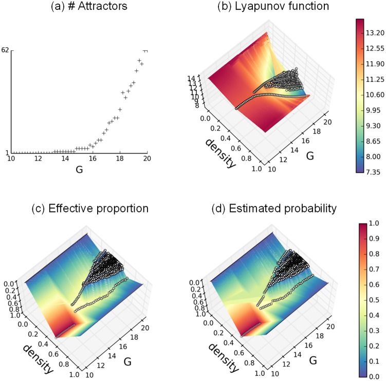
Fig 3. Bifurcation diagrams in the SL model.
a. Number of attractors in function of G. b. Attractors Lyapunov values in function of attractor densities and G. c. Attractors observed proportion in function of attractor densities and G. d. Attractors predicted proportion in function of attractor densities and G, with β = 2. Each distinct attractor in subfigures b-d is denoted by a white dot. The color mappings, interpolated from the discrete values, are provided for enhanced readability. P = 1, G ∈ [10;20].

