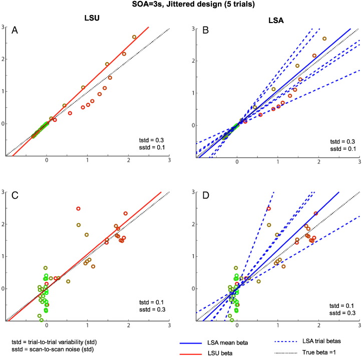
Supplementary Fig. 5.

Comparison between LSU (left panels) and LSA (right panels) for a short SOA (3 s) jittered design of only 5 trials, with either low (top row) or higher (bottom row) scan noise. See legend of Supplementary Fig. 1 for more details, though note that true (population) beta is now 1, for illustration purposes.

Comparison between LSU (left panels) and LSA (right panels) for a short SOA (3 s) jittered design of only 5 trials, with either low (top row) or higher (bottom row) scan noise. See legend of Supplementary Fig. 1 for more details, though note that true (population) beta is now 1, for illustration purposes.

When trial-to-trial variability is higher than the scan noise, as in the upper row, the LSU model in Panel A cannot account for all the variability from trial-to-trial, and some trials (brown colored points) have a greater effect on the best-fitting slope than other trials (red points). The LSA model, on the other hand, can effectively fit a different line to each trial (dashed blue lines), as shown in Panel B, producing a better overall fit (and less affected by more extreme points). When averaging the slopes (Betas) from each trial, one can obtain a more precise estimate of the population mean, as in Fig. 2F of the main paper.

However, when scan noise is higher than the trial-to-trial variability, as in the bottom row, LSA's extra flexibility (higher degrees of freedom) in Panel D means that some of its individual trial estimates fit the scan noise instead. This results in LSA over-fitting the data, and hence its estimate of the population mean (averaging across trials) now becomes less precise than for the more constrained LSU fit in Panel A. Together, this explains why the relative advantage of LSU vs LSA (at short SOA) depends on the ratio of trial variability to scan noise, as shown in Fig. 3 of the main paper.