FIG. 6. Comparing modeled errors in measured pIC₅₀ values using tip-based or acoustic direct dispensing.

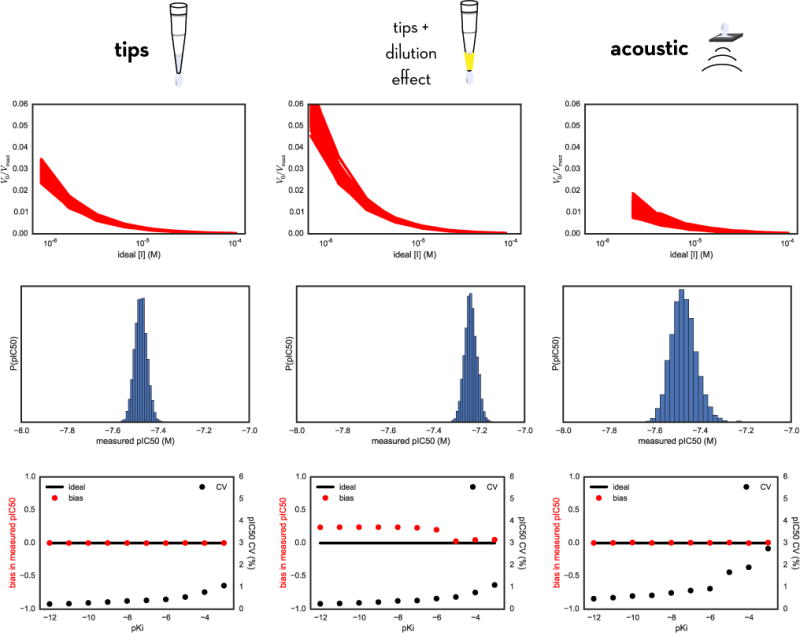
Top row: Bootstrap simulation of the entire assay yields a distribution of V₀/V_max (proportional to measured product accumulation) vs ideal inhibitor concentration [I] curves for many synthetic bootstrap replicates of the assay. Here, the inhibitor is modeled to have a true K_i of 1 nM (pK_i = −9). Middle row: For the same inhibitor, we obtain a distribution of measured pIC₅₀ values from fitting the Using our model we can look at the variance in activity measurements as a function of inhibitor concentration [I] (top), which then directly translates into a distribution of measured pIC₅₀ values. Bottom row: Scaning across a range of true compound affinities, we can repeat the bootstrap sampling procedure and analyze the distribution of measured pIC₅₀ values to obtain estimates of the relative bias (red) and CV (black) for the resulting measured pIC₅₀s. For all methods, the CV increases for weaker affinities; for tip-based dispensing using fixed tips and incorporating the dilution effect, a significant bias is notable.