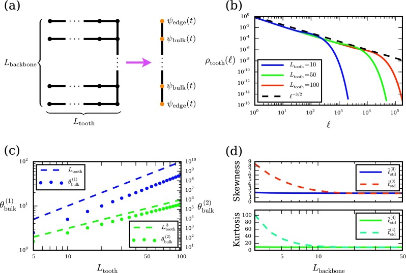
FIG. 3.

Distributions of path lengths and times on a 1D comb. (a) Schematic of a comb with backbone of length L_backbone and teeth of length L_tooth. We coarse-grain the teeth into single states (orange) along the backbone with effective waiting time distributions ψ_edge(t) and ψ_bulk(t). (b) Path length distribution ρ_tooth(ℓ) to exit a tooth of different lengths L_tooth, along with the power law ℓ^−3/2 for comparison. (c) Mean ${\theta }_{\mathrm{bulk}}^{\left(1\right)}$ and second moment ${\theta }_{\mathrm{bulk}}^{\left(2\right)}$ of ψ_bulk(t) as functions of tooth length L_tooth; points are numerical calculations, while dashed lines show expected scaling behavior from Eq. (66). (d) Skewness ${\overline{\ell }}_{\mathrm{std}}^{\left(3\right)}$, ${\overline{t}}_{\mathrm{std}}^{\left(3\right)}$ and kurtosis ${\overline{\ell }}_{\mathrm{std}}^{\left(4\right)}$, ${\overline{t}}_{\mathrm{std}}^{\left(4\right)}$ of length and time distributions for paths along the backbone as functions of L_backbone, with L_tooth = 100.