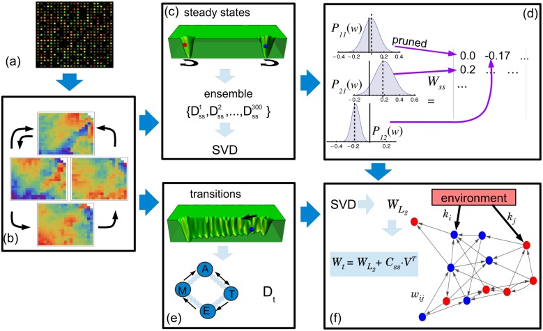
Fig 2. Schema of the network inferring method.

(a) The microarray data corresponding to the parasite’s four steady states are normalised. (b) The total of 8,904 gene-expression levels of each stage is reduced to 339 clusters representing the variables of our systems. (c) An ensemble of 300 training sets including fluctuations around the steady states is constructed from the steady states. Using singular value decomposition (SVD), the minimal L₂-norm solution for each D_ss is determined. (d) A sparse connectivity matrix, W_ss, is derived from the probability distribution P_ij(w) by using a pruning method based on a location test. (e) A new training set is constructed from the transitions between the amastigote (A), epimastigote (E), metacyclic tryp. (M) and trypomastigote (T) stages. Intermediate states (small circles) between the stages are assumed to exist. It is also considered that an unknown external cue (black arrow) is responsible for the transitions. (f) By means of using SVD, the L₂-norm solution, ${\mathbf{W}}_{{\mathbf{L}}_{\mathbf{2}}}$, is determined. This solution is in turn used to find another solution, W_t, which includes information concerning the steady states. This procedure is used to infer the weighted links between genes, w_i,j, and to answer two questions: which genes are affected by the external cues, and how they are regulated (up or down) by the environment.