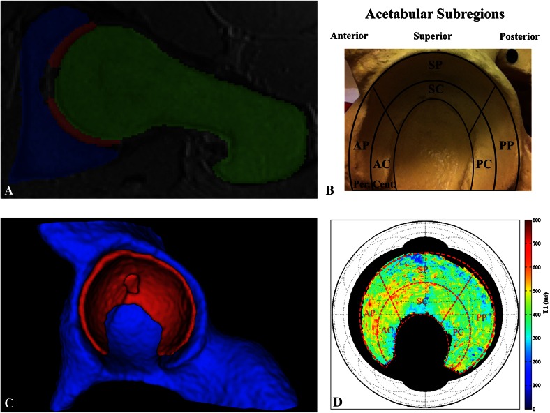
Fig. 1A–D.
(A) The planar dGEMRIC map algorithm [19] takes 3-D, isotropic, 1.5-T dGEMRIC hip sequences and performs automated segmentation of the data to generate the acetabular (blue), cartilage (red), and femoral (green) segments. Shown is a sagittal oblique view of a T1 sequence slice with the segmentation overlay, visualized in ITK-SNAP [22]. (B) The defined acetabular subregions are overlaid on top of a pelvic model for reference. AP = anterior-peripheral; AC = anterior-central; SP = superior-peripheral; SC = superior-central; PP = posterior-peripheral; PC = posterior-central. (C) The cartilage segment (red) is shown, from which the data are extracted and further processed (visualized in ITK-SNAP). Behind it is the acetabular segment (blue), whereas the femoral segment is not shown. (D) Radial averaging and unfolding of the cartilage data yield a planar map that displays the acetabular dGEMRIC signal (visualized in MATLAB, www.mathworks.com). The red, dashed subregion grid from B is overlaid on top of the planar map for clarifying purposes only.

