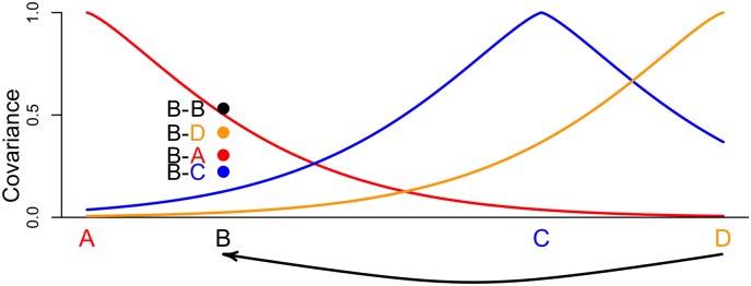
Fig 11. Illustrated example of spatial covariance and the effects of admixture.

Lines show the covariances populations A, C, and D would have with population B as a function of B’s location with no admixture, under the parametric form of Eq (2). The colored dots above ‘B’ show the covariances observed with B at that location given that B has 40% admixture from D. There is no spatial configuration that induces unadmixed covariances remotely similar to those observed.