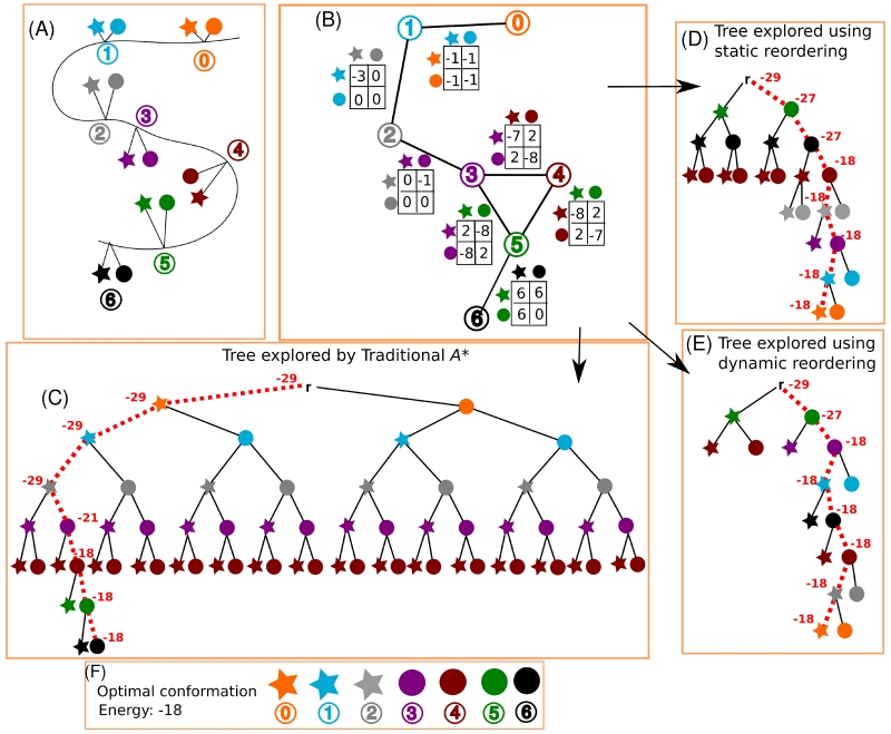
Figure 2. Toy example that demonstrates the effect of residue position reordering on an A* search.

(A) Toy design problem where seven residue positions are each allowed to mutate to two rotamers (represented by a star and a circle). Each residue position is colored by a unique color: orange (position 0), cyan (position 1), grey (position 2), purple (position 3), maroon (position 4), green (position 5), and black (position 6). (B) Diagram showing the pairwise energies between all rotamers in this toy example. For simplicity, assume that all intra-rotamer energies are zero and can be ignored, and that the interactions between pairs that are not joined by an edge are zero. (C-E) The A* algorithm explores only part of the full conformation tree to compute the optimal conformation. A* iteratively expands the node with the lowest f-score (shown by the dotted red path for the nodes in the optimal conformation path) until a leaf is reached. Each expansion results in the creation of new nodes representing the children of the expanded node. To compute the optimal conformation efficiently, it is desirable to expand the fewest number of nodes. The number of nodes expanded can be dramatically reduced by changing the ordering of the tree. (C) The traditional A* algorithm for protein design (Trad-A*) sorts residues in the arbitrary sequential order given by the protein sequence. The bounds on the energies for each inner node in the optimal conformation are shown in red, and the path that leads to the optimal conformation is marked in a thick, red, dashed line. In this toy example, Trad-A* expands 33 nodes, and creates 67 nodes (the 33 expanded nodes plus their children). (D-E) Large speedups in A* can be achieved by a rational ordering of nodes. The energies of each node in the optimal conformation are shown. (D) In a static reordering, residue levels are reordered once before A* runs. In this toy example, A* with static reordering must only expand 13 nodes and create 25 nodes to compute the optimal conformation. (E) In a dynamic reordering, the next level is chosen independently for each path “on the fly” (i.e., as the A* algorithm expands nodes). In this dynamic reordering example, at depth m = 2 the solution path expands position 3 (purple) while the alternative path expands position 4 (maroon). A* with dynamic ordering must expand only 9 nodes, and create a total of 17 nodes, to compute the optimal conformation. (F) The optimal conformation for this example is shown.