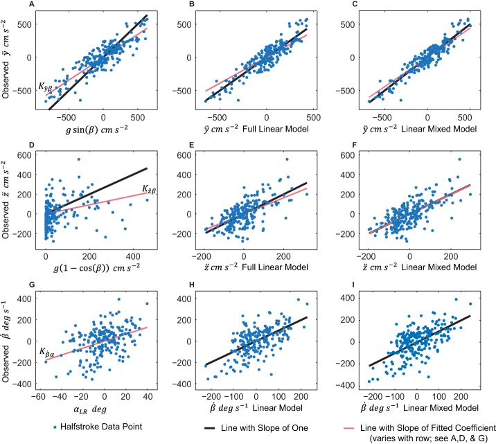
Fig. 1.
Three major moth body position and orientation derivative models. In descending vertical order, rows 1-3 show data for ÿ, z̈, and  . The thin red line has an intercept of zero and a slope equal to the value of the fitted coefficient, (Kÿβ, Kz̈β, and
  respectively by row). The thicker black line has an intercept of zero and a slope of one. In the first column (A,D,G), we fit ÿ and z̈ to the a priori constant dorsally-directed force production model, and
  to αLR (the wing asymmetry that contributed the most to roll velocity). In the second column (B,E,H), we fit ÿ, z̈, and
  to the complete linear models which resulted from the variable selection process (Eqns 6-8). (C,F) We fit ÿ and z̈ to the full linear mixed models; they differ from column two only by the addition of a random intercept for each moth (which resulted in lower AICc values than the models without this adjustment). (H) Linear model for
  , which includes αLR, ΦLR, and
  . (I) Full linear mixed model for
  which differs from panel H by the addition of separate up- and downstroke coefficient estimates for elevation angle. It is important to note that, while we do present this data, panel H scored better than panel I in AICc analysis. n=218 halfstrokes from 19 maneuvers from 4 moths. For P-values see Tables 1 and 3.

