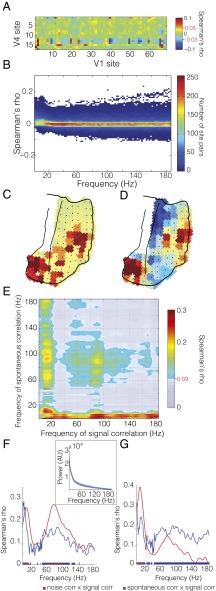
Fig. 4.
Spontaneous correlations. (A) Spontaneous correlation matrix in the gamma band (80–95 Hz) for all V1–V4 site pairs. (B) Distribution of spontaneous correlation values for all interareal site pairs as a function of frequency. Example topographies for spontaneous correlation from the marked V4 site across all visual channels in the (C) theta (6–8 Hz) and (D) gamma (80–95 Hz) bands (same color bar as A). Statistical significance is denoted by red lines and values on color bar, as well as white borders on nonsignificant values in topography. (E) Correlation of interareal spontaneous and signal correlation matrices (A from Figs. 4 and 5) across frequencies. Frequency–frequency plane threshold P < 0.05 corrected for multiple comparisons. Significance threshold is denoted on colorbar by red line and value. (F) Comparison of intrinsic correlations with signal correlations for the gamma frequency band (80–100 Hz). The mean correspondences of spontaneous correlation (in blue) and noise correlation (in red) with signal correlation are shown to illustrate their similar spectral profiles. The line spectra are vertical cuts of the respective frequency–frequency plots shown in Figs. 4E and 5E). Significance threshold at P < 0.05 corrected for multiple comparisons, illustrated in blue and red on the y axis and significant bands of correspondence illustrated as blue and red bars along the x axis. (Inset) Spectrum of absolute power of the normalized raw signal (see Experimental Procedures for details) for the activity during fixation used to compute spontaneous correlation. Mean across visual sites shown in dark blue. Shaded region denotes SD across sites. (G) As in F, but for the low-frequency band (1–20 Hz). The mean correspondences of spontaneous correlation (in blue) and noise correlation (in red) with signal correlation are shown to illustrate their different spectral profiles. The line spectra are vertical cuts of the respective frequency–frequency plots shown in Figs. 4E and 5E). Significance threshold is as explained for F.

