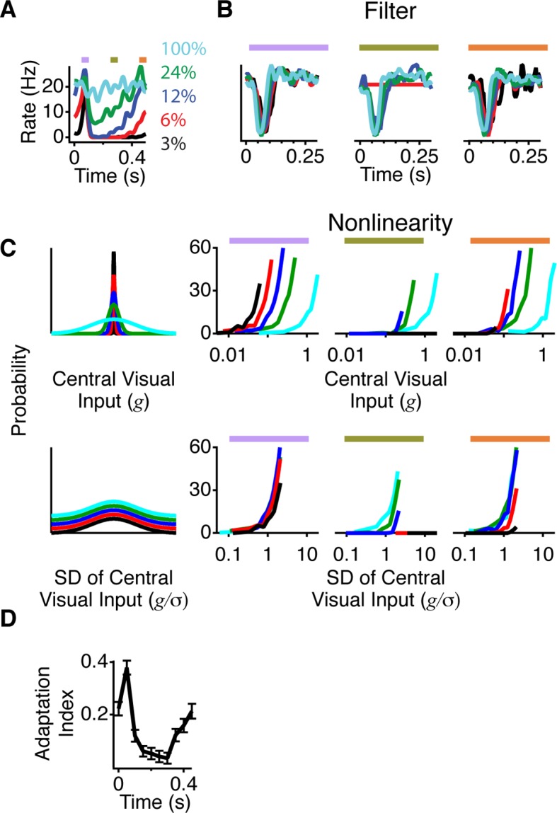
Figure 3. A more adapted representation underlies an increase in information transmission.

(A) The spatial stimulus was the same as in Figure 2. The time course of the central stimulus was a Gaussian white noise stimulus with one of four different contrasts or 100% binary contrast, consisting of black and white intensity values. PSTHs are shown for the different conditions. (B) Filters computed using only spikes from 50 ms time windows, corresponding to color boxes in (A). Purple, gating window; Olive green, suppression window; Orange, recovery window. (C) Input distributions (left) and nonlinearities in the same three 50 ms time windows as in (B). Upper curves are all in units of the linear prediction; lower curves show the same data but in units of standard deviation of the linear prediction. The abscissa is displayed on a logarithmic scale, such that normalization by the standard deviation produces a lateral shift. (D) Average adaptation index across cells that exhibited peripheral excitation (see Materials and methods, n = 400).

DOI: http://dx.doi.org/10.7554/eLife.09266.006

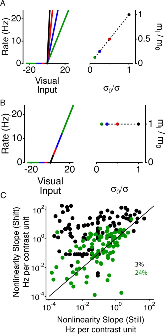
Figure 3—figure supplement 1. Periphery induced changes in adaptation.

(A) Left, schematic nonlinearities for a hypothetical perfectly adapted cell, where the slope of the nonlinear is inversely proportional to the contrast. Right, normalized slope of the nonlinearities vs. normalized inverse contrast, showing the two quantities should be equal for an ideally adapting cell. (B) Same as (A) for a non-adapting cell, showing that for a non-adapting cell the slope does not change. (C) Average nonlinearity slope during the 50 ms time window corresponding to just after the peripheral shift (purple in Figure 3B–D) vs. the average nonlinearity slope during the 50 ms corresponding to the recovery time window (orange) for both high (24%) and low (3%) contrast in the center region.

DOI: http://dx.doi.org/10.7554/eLife.09266.007