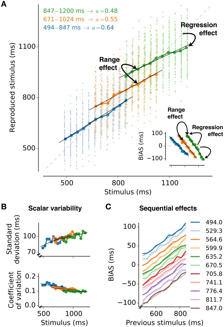
Figure 1.

Psychophysical characteristics of magnitude estimation. The typical properties of magnitude estimation are illustrated as they are reproduced by the model presented in this paper. The description is based on subsecond interval timing (cf., Jazayeri and Shadlen, 2010). (A) Individual reproduced values for each trial and stimulus (small dots, 100 per stimulus value), and their averages (large circles connected by lines) are shown for a simulation with three stimulus ranges. The regression effect is the deviation of the averages from the line of equality (diagonal gray dashed line) toward the mean of the respective stimulus range. It becomes stronger with larger means of the stimulus range, i.e., range effect. The analytical approximation of the model is in line with the simulated data (black solid lines). The memory parameter a was chosen to minimize MSE_r for each range (derived in Section “3.1”). Stimulus ranges and memory weights a are given in the top-left corner of the plot. Other parameters are A_m = A_r = 0.25, σ_m = 1, and σ_r = 0.5. Inset: Average deviations (BIAS) from the line of equality for each stimulus and test range. Solid lines are again analytical predictions. (B) Standard deviation and coefficient of variation (standard deviation divided by the mean) corresponding to (A). Black solid lines are again analytical predictions. (C) Sequential effects. Plotting the response bias for a certain stimulus as a function of the stimulus in the previous trial, reveals effects of stimulus order in the simulations (thick lines). The simulation results can be analytically approximated (thin lines). Results for the range 494 − 847 ms are displayed. For each stimulus value 10,000 trials were simulated.