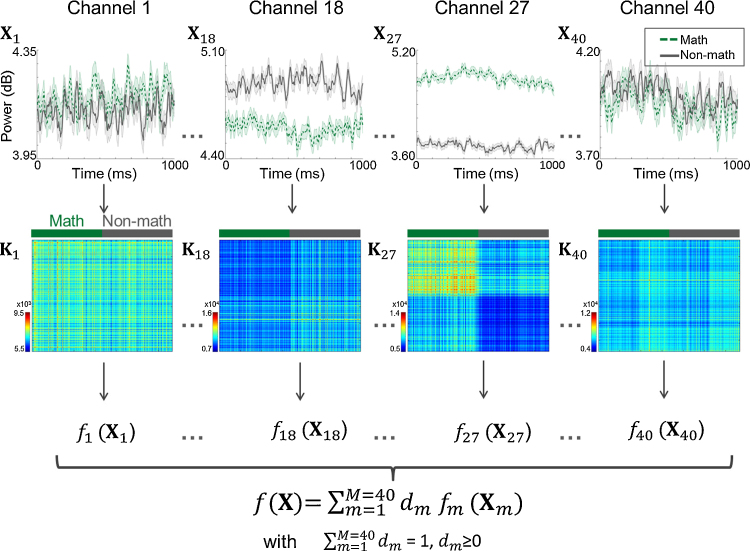
Fig. 2.

Illustration of the multiple kernel learning (MKL) approach considered. For each electrode, the time course of the power in a specific frequency band (here high-γ) is extracted for each trial in the [0 1 0 0 0] ms window around onset. The top row of the figure displays such features averaged across math (dashed green) and non-math (gray) trials (patient P1, session 1), with normalized standard error (shaded areas). From those features, a linear kernel is built for each electrode, as illustrated in the middle row of the figure (trials sorted by category, with Math trials in the top left corner). This matrix is symmetric and displays whether trials from one category are more similar to one another than to trials from another category (as is the case for kernels K₁₈ and K₂₇ but not for kernels K₁ and K₄₀). For each kernel, the model estimates a decision function f_m (m = 1…M, M being the number of electrodes) which is then weighted according to a positive or null contribution d_m. The final decision function is the linear combination of the different decision functions estimated on each electrode. The contributions of all electrodes must satisfy the constraints of summing to 1, and being positive or null, which leads to a sparse selection of electrodes contributing to the final model. (For interpretation of the references to color in this figure legend, the reader is referred to the web version of this article).