. 2015 Nov 2;4:e08998. doi: 10.7554/eLife.08998

Figure 2. The fitted model explains the observed spiking responses, with estimated modulators that are both anatomically and functionally targeted.

(a) Performance comparison of various submodels, measured as log-likelihood (LL) of predictions on held-out data. Values are expressed relative to performance of a stimulus-drive-only model (leftmost point), and increase as each model component (cue, slow drift, and different numbers of shared modulators) is incorporated. The grey square shows the predictive LL for a two-modulator model, with each modulator constrained to affect only one hemisphere (i.e. with coupling weights set to zero for neurons in the other hemisphere). This restricted model is used for all results from Figure 2d onwards, excepting the fine temporal analysis of Figure 6c. (b) Modulators are anatomically selective. Inferred coupling weights for a two-modulator model, fit to a population of units recorded on one day. Each point corresponds to one unit. As the model does not uniquely define the coordinate system (i.e. there is an equivalent model for any rotation of the coordinate system), we align the mean weight for LHS units to lie along the positive x-axis (see Materials and methods). (c) Distribution of inferred coupling weights aggregated over all recording days indicates that each shared modulator provides input primarily to cells in one hemisphere. (d) Hemispheric modulators are functionally selective. Units which are better able to discriminate standard and target stimuli in the cue-away condition have larger coupling weights (blue line). Discriminability is estimated as the difference in mean spike count between standard and target stimuli, divided by the square root of their average variance (d′). Values are averaged over units recorded on all days, subdivided into five groups based on their coupling weights. Shaded area denotes ±1 standard error. Pearson correlation over all units is = 0.42. This relationship is not seen for the weights that couple neurons to the slow global drift signal (gray line, Pearson correlation r = 0.00). The relationship between d′ and cue weight is significant, but weaker than for modulator weight (r = 0.24); this is not shown here as the cue weights are differently scaled. (e) Same as in (d), but with units subdivided into subgroups according to mean firing rate. Each line represents a subpopulation of ∼500 units with similar firing rates (from red to blue: 0–7; 7–12; 12–17; 17–25; 25–35; 35–107 spikes/s). Within each group, the Pearson correlations between d′ and coupling weight are between 0.2–0.3, but the correlations between mean rate and coupling weight are weak or negligible.

DOI: http://dx.doi.org/10.7554/eLife.08998.006

Figure 2.

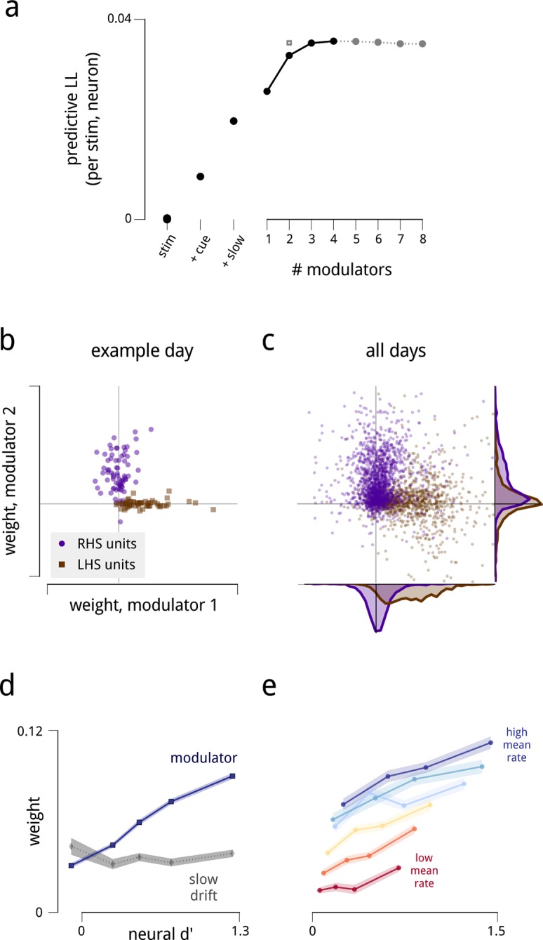
Figure 2—figure supplement 1. The dataset is sufficient to support the estimation of up to 8 shared modulators.

Figure 2—figure supplement 1.

To test whether the number of recovered modulators is limited by insufficiency of the dataset, we simulated data from model neural populations that were under the influence of different numbers of modulators. All simulated datasets were matched in size to the physiological data, and simulated shared gain fluctuations were adjusted in amplitude to produce the same pairwise spike count statistics as the actual data. We then fit the model to these synthetic datasets, and measured how well the model fits recovered the true modulatory structure. More specifically, we extracted default model parameters by fitting each neural population: the stimulus-driven mean firing rates F, the cue-dependent gains C, and the slow global drifts D. Then, for a given number of simulated modulators K (from 1 to 12), we sampled a (T × K) matrix of time-varying modulator values (each value i.i.d. Gaussian), and a (K × N) matrix of random weights (each weight i.i.d. Gaussian), producing a net modulator matrix M as the matrix product of these two. We then sampled spike counts Y from the generative model, Y~Poiss(F1Texp(C+D+λM)). For each population and K, we chose the scaling parameter λ such that the median noise correlation between the simulated neurons matched the median noise correlation between the actual neurons. We next fitted the models to these simulated datasets to see how well they recovered the underlying structure. As for the actual data (Figure 2), we evaluated the model fits via the predictive log-likelihood on held-out data. Each colored line shows the predictive LLs of the fitted models for a given “ground truth” number of modulators. In comparison, the grey squares show the model performance for the actual data. There are two important patterns here. First, for simulated models containing up to 8 modulators, the predictive LLs are greatest when we fit a model having the same number of modulators as the ground truth number used to simulate the data. This demonstrates that the model is in principle able to recover more modulators than the 4 we fit to the actual data. Second, as the number of simulated modulators increases, the ability of the fitted models to make predictions on held-out data declines. This is because the total energy of the shared gain fluctuations is constrained by the measured noise correlations, and is spread amongst the simulated modulators. In this respect, the model predictions on the actual data are most consistent with simulations of 3 or 4 modulators. Finally, it is worth noting that, in simulation, when fitting more modulators than the ground truth, the predictive performance suffers. This reflects overfitting to the noise in the training set. We do not see as pronounced a decline for the model fits to the actual data: instead, the predictive LLs appear to saturate with the number of modulators. This difference between the actual and synthetic data likely reflects our assumption in the simulations that the modulators were all of equal magnitude. A saturation of predictive LL may arise when there is a small set of dominant modulators, and a number of weaker ones. We do not have the statistical power to explore such a long tail of modulatory influences within this dataset, and focus instead on the strongest components.
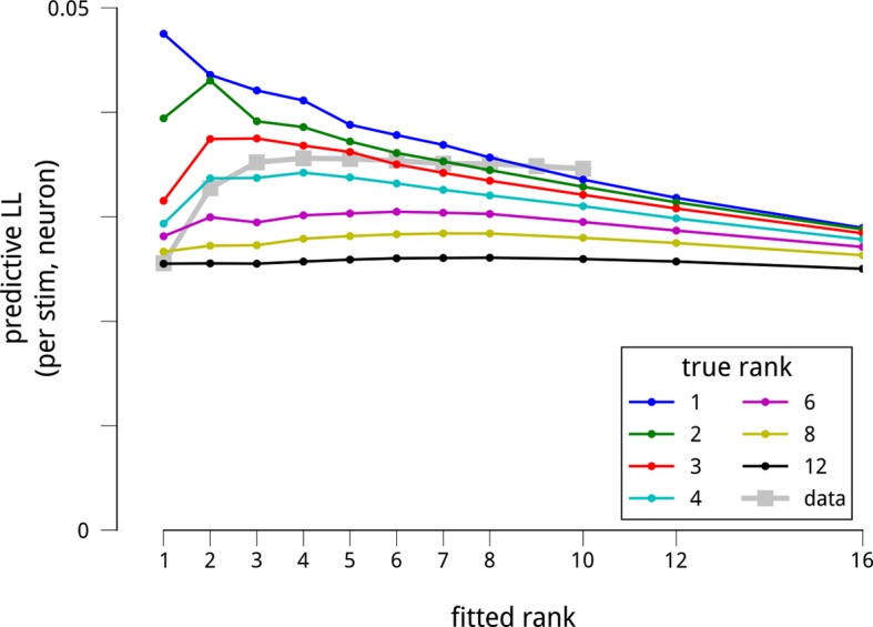
Figure 2—figure supplement 2. The structure of the modulators in higher-dimensional modulator models.

Figure 2—figure supplement 2.

In the main text, we identify three striking properties of the two dominant shared modulators: (1) they each target one of the two V4 hemispheres; (2) they preferentially target the task-specific neurons within these hemispheres; and (3) their variance decreases under cued attention. Here we show that these features are present within higher-dimensional modulator models. In Figure 2—figure supplement 3, we show that these additional modulatory components do not convey any additional structure in these three domains. It is useful to first view the modulator model as a form of exponential-family Principal Component Analysis (PCA) (Collins et al., 2001; Solo and Pasha, 2013;Pfau et al., 2013). Standard PCA, like the shared modulator model, uncovers directions in signal space of maximal variation. However, PCA suffers from an identifiability problem: it can uniquely recover the subspace in which a small set of signals lie, but not the coordinate axes. PCA does select a particular orthogonal coordinate system to represent this subspace, but this solution is not unique, is sensitive to noise, and typically reveals little about the underlying generative process. This same identifiability problem is present with the shared modulator model. In the two-modulator case, we are able to resolve the ambiguity in the coordinate system by exploiting anatomical information (Figure 2b–c; see Materials and methods). However, the problem of identifiability becomes more acute in higher dimensions. Here, we show that the results presented in the main text for the 1-modulator/hemisphere model also hold for the unconstrained 2-modulator model. We also extend the 2-modulator results to the 3- and 4-modulator cases. This is necessary as, unlike standard PCA, the solutions to our equations in lower dimensions do not necessarily lie within subspaces of higher-dimensional solutions. This is because the regularization scheme and algorithm we use create biases that disrupt any strict nesting. We therefore need to explicitly test whether the structures we uncover in the 2-modulator model are also present in the 3- and 4-modulator models. And this needs to be done under the limitations of the identifiability problem, i.e. without choosing a particular coordinate system for the modulation subspace. First column: In Figure 2b–c, we showed that the vectors of modulator coupling weights for LHS units and RHS units in the 2D modulator model were typically orthogonal. Here we show that this holds in higher dimensions. For each recording day, we measured the angle between the average weight vector for LHS units (w¯L), and the average weight vector for RHS units (w¯R), i.e. the arc cosine of their inner product. The 2-modulator hemisphere-constrained model used in most of the main text has this orthogonality enforced by constraint (top row). For the unconstrained 2-, 3-, and 4-modulator models (remaining rows), the blue histograms show the distribution of these angles across recording days. For comparison, we shuffle the anatomical labels on each unit and repeat the analysis to obtain the red histograms. The clustering of the actual data around π/2 indicates near orthogonality of the hemispheric weights. Second column: In Figure 2d, we showed that neurons which were task-relevant (i.e. had larger d′ values) were more strongly coupled to the (1D) hemispheric shared modulators. Here, we show that this holds in higher dimensions. For each recording day, we measured the magnitudes of all units’ coupling weight vectors, w2. Green histograms show the distribution of magnitudes for the quartile of units with largest d′ values; brown histograms show the distribution of magnitudes for the quartile with the smallest d′ values. Third column: In Figure 3b, we showed that the variance of the (1D) hemispheric shared modulators changed according to the attentional cue: specifically, when the cue switched, one hemispheric modulator decreased in variance, while the other increased in variance. To show that this holds in higher dimensions, it is necessary to construct an appropriate metric for this change in second-order statistics that generalizes to higher dimensions, and that also does not depend on a choice of coordinate system. To accomplish this, we measure the effect of the attentional cue as a change in the covariance of the (multivariate) modulator. Considering the change from the cue-right to the cue-left condition, we can measure the effect on the modulator’s second-order statistics via the ratio of the two modulator covariances, CcueLCcueR-1. The eigenvalues of this matrix then provide a coordinate-system-free measure of how the modulator statistics change. If the largest eigenvalue, λmax, is significantly greater than 1, then there is a direction in modulation space that became more variable due to the switch in cue. If the smallest eigenvalue, λmin, is significantly less than 1, then there is a direction in modulation space that became less variable due to the switch in cue. Eigenvalues close to 1 indicate that the variance of modulation in that direction was unchanged by the cue. Thus these two values, λmax and λmin, play an analogous role to the ratios of modulator variance examined in Figure 3b. The scatter plots show the distribution of λmax and λmin for the higher-dimensional modulator models. Blue points show these eigenvalues from each recording day; red points show the distributions obtained if we shuffle the cue labels for each trial. Importantly, when λmax exceeds 1 and λmin is less than 1 (i.e. when the points lie in the lower right quadrant), then the change in attentional cue is causing an increase in modulator variance in one direction, and a decrease in modulator variance in an orthogonal direction. These effects are clear (and significant, compared with the null distribution in red) in all cases.
Figure 2—figure supplement 3. The modulators' anatomical, functional, and attentional structure manifests primarily within the dominant two dimensions of modulation.

Figure 2—figure supplement 3.

In the main text, we recover a set of anatomical, functional, and attentional properties within a 2-dimensional modulator model. In Figure 2—figure supplement 2, we demonstrate that these properties also manifest within 3- and 4-modulator models. We wondered whether any additional structure can be seen in the extra two dimensions of modulation that we can include beyond the 2-modulator model. To answer this, we partitioned the 4-dimensional modulator space into two 2-dimensional halves. For each recording day, we define a particular 2D subspace of modulation along anatomical grounds. We measured the mean weight vectors for LHS and RHS units, w¯L and w¯R respectively. As shown in Figure 2—figure supplement 2, these two vectors were always near-orthogonal. We define their 2D span as the “hemispheric subspace of modulation”, H=span(w¯L,w¯R). This is a 2D subspace of the 4D weight vectors, capturing the largest component of hemispheric-specificity in the modulator weights. What remains in the 4D modulation space is the hemispheric subspace’s orthogonal complement, H. This divides the 4D space into two 2D subspaces, and thus amounts to a partial choice of a coordinate system. We can therefore study the anatomical and functional properties of the coupling weights in H and H, and also the attention-dependent statistics within the corresponding 2D spaces of time-varying modulator values. This panel shows that all three properties described in Figure 2—figure supplement 2 manifest predominantly in H, but not in H. In summary, each V4 hemisphere is being driven by a shared modulatory signal, that preferentially affects task-specific neurons, and has statistics that depend on the attentional cue provided to the animal. In addition, there is some evidence that other shared modulatory factors are affecting the population of V4 neurons. However, these latter signals do not share the same properties: their net effects are weaker, they do not appear to have the same anatomical or functional specificity, and they do not appear to be affected by the attentional cue.
Figure 2—figure supplement 4. Units with higher mean firing rates typically had stronger coupling to their respective population modulator (r2 = 0.21).

Figure 2—figure supplement 4.

This observation motivates the control analyses shown in Figure 2e, Figure 5—figure supplement 1 and Figure 8—figure supplement 1.