Estimating daily air temperature across the Southeastern United States using high-resolution satellite data: a statistical modeling study

Abstract

Accurate estimates of spatio-temporal resolved near-surface air temperature (T_a) are crucial for environmental epidemiological studies. However, values of T_a are conventionally obtained from weather stations, which have limited spatial coverage. Satellite surface temperature (T_s) measurements offer the possibility of local exposure estimates across large domains. The Southeastern United States has different climatic conditions, more small water bodies and wetlands, and greater humidity in contrast to other regions, which add to the challenge of modeling air temperature. In this study, we incorporated satellite T_s to estimate high resolution (1 km × 1 km) daily T_a across the southeastern USA for 2000-2014. We calibrated T_s to T_a measurements using mixed linear models, land use, and separate slopes for each day. A high out-of-sample cross-validated R² of 0.952 indicated excellent model performance. When satellite T_s were unavailable, linear regression on nearby monitors and spatio-temporal smoothing was used to estimate T_a. The daily T_a estimations were compared to the NASA's Modern-Era Retrospective Analysis for Research and Applications (MERRA) model. A good agreement with an R² of 0.969 and a mean squared prediction error (RMSPE) of 1.376 °C was achieved. Our results demonstrate that T_a can be reliably predicted using this T_s-based prediction model, even in a large geographical area with topography and weather patterns varying considerably.

1. Introduction

Global warming adds urgency to better understand the impact of temperature on health, particularly in the warm areas such as the southeastern USA. Growing evidence has linked near-surface air temperature (T_a), an important environmental stressor, with morbidity and mortality (1-7). Previous studies concerning human health and T_a exposure are primarily limited by the spatial and temporal availability of T_a measurements, leaving large areas uncovered. Temperature can vary greatly both in space and time, therefore these collected point-samples are insufficient to adequately capture the spatial and temporal variability within a large area (8). In addition, owing to the urban heat-island effect, higher temperatures are often observed in urban areas versus surrounding areas. For example, temperatures measured in a station near an airport may underestimate the true near-surface air temperatures in the urban area.

However, these small geographic changes in air temperature can have important health effects. Shi et al. (2015) found that both geographical contrasts and annual anomalies of local air temperature contribute to excess public health burden of climate change (9). They used daily local air temperature estimates at fine geographic scale (1 km × 1 km) in New England, to capture the exposure variability in space and time which may be driving the adverse health effects. Lower exposure measurement errors, and the inclusion of the entire region, largely alleviate the downward bias in health effect estimates.

In recent years, several methods were developed to address the lack of high-resolution exposure data. Geospatial statistical methods, such as land use regression and kriging, are most commonly used approaches. They allow characterizing the spatial heterogeneity of exposure by using time invariant geographical variables to expand the ground monitored measurements to large areas (10, 11). However these methods do not generally capture temporal variability in exposure, in that they are commonly based on a year of intensive monitoring, and miss changes over years in the spatial pattern of T_a. Therefore they are primarily used to assess chronic health effects.

Satellite-based remote sensing can provide additional information at high spatial and temporal resolution. Satellite instruments, such as Moderate Resolution Imaging Spectroradiometer (MODIS), can provide global daily estimates of 1 km surface skin temperature (T_s), the temperature at the air-soil interface (12-14). T_s is derived from the thermal infrared signal received by the satellite sensor. T_s as an indicator of the net surface energy balance, depends on the presence of vegetation or plant cover, atmospheric conditions, and thermal properties of the underlying surfaces. It is different from T_a, which is measured at meteorological stations at the screen height of 1-2 m above the land surface.

Several studies have shown that T_s and T_a are correlated (15, 16). Even so, there are many factors that can influence the complex and geographically heterogeneous relationship between T_s and T_a, such as humidity, the type of underlying surfaces, the elevation, and other surface parameters. Additionally, Dousset (17) stated that T_a has superior correlation with T_s at night because the solar radiation does not affect the thermal infrared signal. During nighttime T_s is close to T_a and during daytime T_s is generally higher than T_a (12).

The value of T_a cannot be predicted by T_s using a simple linear relationship with reasonable accuracy. Fu et al. (2011) explored predicting T_a using satellite T_s and found an R²>0.55 (18). Recently, Kloog et al. (2014) presented a novel model and assessed daily mean T_a in the northeastern USA using MODIS-derived T_s measurements (19, 20). Better predictive performance was reported. For days with available T_s data, mean out-of-sample R² was 0.947. Even for days without T_s values, the model accuracy was also excellent. Although T_a estimation in the northeastern USA was excellent, it is uncertain that how well the satellite approach would perform in areas with different geographic features and weather patterns.

Predicting T_a for the southeastern USA is of top priority for epidemiological studies. Many researchers are of great interest in investigating the health effects of temperature using the Medicare cohort (aged 65+), because this elderly population is potentially most vulnerable to climate change. Due to its warm weather, the southeastern USA contains a very large Medicare population (13 millions). Thus, it is particularly urgent to provide a comprehensive temperature dataset for this particular region.

The aim of this paper was to estimate 15-year daily local air temperature in the southeastern USA, by extending and validating the previous hybrid-model approach to account for the unique geographical and climatological characteristics of the study area. Specifically, by incorporating satellite derived T_s, T_a measured at monitors, meteorological variables and land use terms, we employed a 3-stage statistical modeling approach to obtain daily air temperature predictions at 1 km × 1 km resolution across the southeastern USA for the years 2000-2014. The retrieved air temperature was cross validated against the measurements from weather stations. As an independent validation, the results were also compared with NASA's reanalysis products, Modern-Era Retrospective Analysis for Research and Applications (MERRA).

2. Materials and Methods

2.1 Study domain

The spatial domain of our study includes the southeastern part of the USA, comprising the states of Georgia, Alabama, Mississippi, Tennessee, North Carolina, South Carolina and Florida (Fig. 1). The southeastern states include some populous metropolitan areas (Charlotte, Memphis, Raleigh, Atlanta and Miami), rural towns, large forested regions, mountains, water bodies, and the Atlantic sea shoreline. The study region covers an area of 916,904 km² with a population of 56,742,948 according to the 2010 census (UCSB, 2010), and encompasses 1,013,408 discrete 1 km × 1 km satellite grid cells.

Fig. 1.

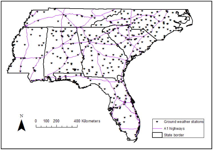
Map of the study area showing all available NCDC air temperature monitor stations across southeastern USA for 2000-2014.

2.2 Surface temperature

Daily T_s data from the MODIS sensors located on polar orbiting Terra satellite for the years 2000-2014, with a spatial resolution of 1 km × 1 km were used to prepare the analysis presented in this paper. They were calculated from land surface temperature (LST) and emissivity using the formula T_s =LST/Emissivity^1/4. These MOD11_A1 products (LST & emissivity) are freely available online through the NASA website (NASA, 2014), and cover tiles h10v05, h10v06, and h11v05. They include the latitude and longitude of 1 km grid cell centroid, nighttime and daytime LST, and emissivity.

Nighttime T_s was observed to have a higher correlation with air temperature (r = 0.94), compared to daytime T_s (r = 0.87). This is consistent with previous literature, demonstrating that the nighttime T_s generally present superior correlations with ground measurements of T_a across most sites in the USA. More details about MODIS T_s data can be found in the literature (19, 21).

2.3 Meteorological data from weather stations

In our analysis, daily data for T_a from weather stations across the southeastern USA (see Fig. 1) for 2000-2014 were obtained from the National Climatic Data Center (NCDC). There were 538 NCDC stations operating daily in the southeastern USA during the study period. The mean T_a across the study area during the study period was 18.59 °C with a standard deviation of 7.96 °C and an interquatile range (IQR) of 12.28 °C.

2.4 NDVI

The presence of vegetation on the surface can also affect T_s, since incoming solar radiation is partly intercepted by vegetative surfaces during the day, and part of the outgoing longwave radiation at night is also intercepted by vegetation. Normalized Difference Vegetation Index (NDVI) data were available at 1 km resolution from the monthly MODIS product (MOD13A3). Monthly vegetation index was used as NDVI values have little within-month variation and the spatial distribution is illustrated in the Appendix A (Fig. A.1). To create the covariate of NDVI for daily T_s. the distances between centroids of NDVI and that of a grid cell of T_s were calculated, and the nearest NDVI value of the current month was merged.

2.5 Spatial predictors of air temperature

To enhance the predictive ability of the final model, we included the following statistically significant spatial predictors in the models, which influence T_s or T_a and thereby modify the relationship between T_s and T_a. These time-invariant variables were first processed into 1 km × 1 km spatial resolution (details are described below). Spatial distributions for these variables are illustrated in the Appendix A (Fig. A.2 – Fig. A.4). For the daily dataset, spatial predictors were assigned to the nearest grid cell for each day, and these data served as covariates for the daily surface temperature.

2.5.1 Percent of urban areas

In urban areas, residential, commercial and industrial developments often produce radical changes in radiative, thermodynamic and aerodynamic characteristics of the surface. Thus the associated T_s are often modified substantially. Percent of urban areas data were obtained from the 2011 national land cover data (NLCD) (22). Data were available as raster files with a 30 m spatial resolution. We reclassified the raster into 0 (open space) and 1 (urban areas), by recoding land cover codes 22, 23, 24 (sub categories for developed areas) to 1 as an urban cell and assigning 0 for the remaining. The mean of the 30 m-resolution binary values within each 1 km grid cell was calculated, namely percent of urban areas.

2.5.2 Elevation

There are notable elevation contrasts across such a large area, thus elevation was used as a spatial predictor. Generally, higher elevations are associated with lower air temperatures. Elevation data were obtained from the National Elevation Dataset (23). NED data is available from the U.S. Geological Survey (USGS) and provides elevation data covering the Unite States at a spatial resolution of 1 arc second (30 m). The mean of the 30 m-resolution elevation values within each 1 km grid cell was calculated and used as a spatial predictor.

2.5.3 Distance to water body

The presence of moisture at the surface greatly moderates the diurnal range of surface temperatures, due to the increased evaporation from the surface and increased heat capacity of water. Over a free water body, about 80% of the net radiation is utilized for evaporation on average and the ground heat flux is reduced. We used the Esri Data and Maps for ArcGIS 2013 for water body data. We created a dummy variable taking the value of 1, if the 1 km grid cell centroid is on water and 0 otherwise. The distance from centroids to water body (a continuous measure) was also calculated, which equals to 0 if the centroid is on water.

2.6 Statistical methods

Data preparation was implemented using MATLAB (R2014b, MathWorks), and all modeling was done using the R statistical software. The prediction process consists of 3 stages. The stage 1 model calibrates the T_s - T_a relationship on each day during 2000-2014 using data from grid cells with both ground T_a monitors and T_s measurements. We performed daily calibrations with nighttime MODIS T_s for the reasons noted earlier. The base model (stage 1), fit to data from each year (2000-2014) separately, consists of a mixed model with day-specific random effects to capture the day-to-day variation in the T_s - T_a relationship. Specifically the base model can be written as:

$$T_{aij}=(\mathrm{\alpha }+{\mathrm{u}}_j)+({\mathrm{\beta }}_1+{\mathrm{V}}_j)T_{sij}+{\mathrm{\beta }}_2{\text{Elevation}}_i+{\mathrm{\beta }}_3{\text{NDVI}}_{ik}+{\mathrm{\beta }}_4{\text{Percent urban}}_i+{\mathrm{\beta }}_5{\text{Distance to water body}}_i+{\mathrm{\beta }}_6{\text{water body}}_i+{\mathrm{\epsilon }}_{ij}$$

(u_j v_j) ∼N[(0 0), Σ]

where T_aij denotes the measured mean air temperature at a spatial site i on a day j; α and u_j are the fixed and random (day-specific) intercepts, respectively, T_sij is the surface temperature value in the grid cell corresponding to site i on a day j; β₁ and v_j are the fixed and random slopes, respectively. Elevation_i is the mean elevation in the grid cell corresponding to site i, NDVI_ik is the monthly NDVI value in the grid cell corresponding to site i for the month in which day j falls, percent urban_i is the percent of urban area in the grid cell, distance to water bodyi is the distance of the grid cell to the nearest water body, and water body_i is a 0/1 dummy variable identifying grid cells that intersect water polygons. Finally, Σ is an unstructured variance-covariance matrix for the random effects and ε_ij is the error term at site i on a day j.

The performance of the base model was validated by 10-fold cross-validation. The dataset was randomly divided into 90% and 10% splits ten times. We fit the model using 90% of the data, and then use this model to predict for the held-out 10% of the data. Then the “out-of-sample” cross-validated (CV) R² were computed. To check for bias, we regressed the measured T_a values in the held-out data against the predicted values in each site on each day. We assessed the model prediction performance by taking the square root of the mean squared prediction errors (RMSPE). Overall temporal R² and overall spatial R² were calculated as well. More details are provided in Kloog et al. (20).

In stage 2, we predicted T_a in grid cells without monitors but with available T_s measurements using the stage 1 model coefficients. This is implemented by simply applying the estimated prediction model fit obtained from stage 1 to these additional T_s values. This resulted in datasets with T_a predictions for all available T_s cell/day combinations.

To impute data for grid cells/days for which T_s measurements were not available, the stage 3 model was fitted by using the stage 2 predictions. Specifically, for each grid cell, we regressed the T_a predictions obtained from stage 2 on the daily mean measured T_a (from the stations within a 100 km buffer of that grid cell), land use terms and a smooth nonparametric function of latitude and longitude of the grid cell centroid, with random cell-specific intercepts and slopes. This is similar to universal kriging, by using T_a measurements from nearby grid cells to help fill in the missing. We selected a 100 km buffer size because it was small enough to ensure relevance and large enough to include multiple T_a stations to produce more stable estimates. Because the spatial patterns of T_a vary temporally, a separate spatial surface was fit for each two-month period. This approach provides additional information about the T_a in the missing grid cells that simple kriging would not. Specifically, the following semiparametric regression model was fitted:

$$\text{pred}{T}_{aij}=(\mathrm{\alpha }+{\mathrm{u}}_j)+({\mathrm{\beta }}_1+{\mathrm{v}}_j)\mathrm{m}{T}_{aij}+{\mathrm{\beta }}_2{\text{NDVI}}_{ik}+{\mathrm{\beta }}_3{\text{Percent urban}}_i+{\mathrm{\beta }}_4{\text{Distance to water body}}_i+\text{Smooth}{(\mathrm{X},\mathrm{Y})}_{\mathrm{k}(j)}+\text{Bimon}+{\mathrm{\epsilon }}_{ij}$$

(u_j v_j) ∼ [(0 0), Ω_β)]

where PredT_aij is the predicted air temperature at a grid cell i on a day j from the mixed model; mT_aij is the mean T_a in the relevant 100 km buffer for cell i on a day j; α and u_j are the fixed and random intercepts, respectively; β₁ and v_i are the fixed and random slopes, respectively. NDVI_ik is the monthly NDVI value in the grid cell corresponding to site i for the month in which day j falls, percent urbani is the percent of urban area in the grid cell, and distance to water body_i is the distance of the grid cell to nearest water body. The smooth (X,Y) is a thin plate spline fit to the latitude and longitude of the centroid of grid cell i, k(j) denotes the two-month period in which day j falls (that is, a separate spatial smooth was fit for each two-month period).

The calculated coefficients of the stage 3 model would then be used to fill in the missing T_a values. In contrast to stage 2, the stage 3 model includes cell-specific random intercepts and slopes, which allows for temporal and spatial interpolation for each grid cell. That is, we could use the random effects for a grid cell to help impute T_a data of this cell for days when T_s measurements were unavailable. If grid cells did not have any temperature monitors within their 100 km buffer, no temperature was imputed. Such locations were generally in unpopulated areas.

2.7 Validation against reanalysis data

MERRA is a NASA reanalysis dataset generated using the version 5.2.0 of the Goddard Earth Observing System (GEOS-5) atmospheric data assimilation system. Reanalysis is a technique for generating a comprehensive meteorological record by assimulating observations from multiple platforms using numerical models. Different from the statistical approach used in this study, the models used in reanalysis are based on physical rules of atmospheric motions. The reanalysis datasets are widely used for analysis of long term, large scale climatic changes. Their spatial resolution, however, is usually coarse (24). Although reanalysis may also utilize some of the observations, such as the weather station data and satellite irradiance, which are also used in the statistical modeling, it represents an entirely different modeling approach and its results can be considered as an independent source of information for validation purpose.

In this study, the MERRA daily air temperature at 2 m above displacement height (T_2m) was chosen to validate the retrieved T_a. MERRA data has a coarser spatial resolution of 1/2° × 2/3° in latitude/longitude. The 1 km grids of retrieved T_a were matched with the nearest MERRA grid centroid. A MERRA grid can contain 3000 to 4300 of such 1 km grids. These grids were aggregated and averaged by day, and the averaged data were used for validation. For some MERRA grids which contain both land and ocean pixels, the number of matched 1 km grids can be less, because our statistical model only retrieves air temperature above the land. To avoid interference of ocean pixels, MERRA with less than 1878 (lowest 15^th percentile) 1 km grids matched were removed from analysis.

3 Results

The correlation between the satellite-derived T_s and the T_a obtained from the monitor sites within the same grid cells was high, indicating that T_s can provide useful information for predicting T_a. As an example, results for the year 2011 are shown in Fig. 2 (left). An R² value of 0.89 indicates that although T_s and T_a are highly correlated, there are still some variations of T_a cannot be explained by T_s without the calibration using more predictors. Other factors, such as elevation, NDVI, and land use terms can also affect the T_a - T_s relationship. Their correlations with T_a and T_s are shown as well (see Table A.1 and A.2). Taking those factors into account, the relationship between the predicted T_a from our daily calibration method and the monitored T_a is greatly improved (e.g., R²=0.96 in 2011). Effect estimates for stage 1 are reported in Appendix A (Table A.3).

Fig. 2.

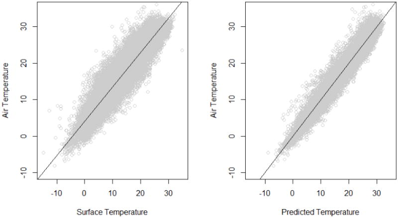
Scatter plots of the monitored air temperature versus satellite surface temperature (left) and the monitored air temperature versus that from the stage 1 calibration (right). Data are shown for the year 2011.

For the stage 1 calibration, we conducted a 10-fold cross-validation. The results of 10-fold cross-validation, which can represent the out-of-sample performance of our stage 1 model, are presented in Table 1. For the entire study period, the mean out-of-sample R² was 0.952 (year-to-year variation 0.935 -0.962). The spatial and temporal R² values (mean of 0.867 and 0.961, respectively) also showed good performance of the model. We found no bias in our cross-validation results (slope of observed versus predicted = 1.00). The model also yielded small prediction errors, with an RMSPE of 1.662 °C and spatial RMSPE of 0.903 °C. All of these indicated excellent model performance. To show the heterogeneity of the model performance, the results of 10-fold cross-validation for each state for the year 2011 are reported in Appendix A (Table A.4).

Table 1. Prediction accuracy in Stage 1: 10-fold cross-validated (CV) R² for daily T_a predictions (2000-2014).

Year	CV R2	CV R2Spatial	CV R2Temporal	RMSPE	RMSPESpatial
2000	0.941	0.804	0.955	1.74	1.071
2001	0.937	0.860	0.948	1.796	0.973
2002	0.962	0.888	0.970	1.530	0.871
2003	0.944	0.840	0.955	1.753	0.942
2004	0.943	0.858	0.953	1.804	0.938
2005	0.960	0.854	0.971	1.541	0.888
2006	0.935	0.792	0.942	1.920	0.977
2007	0.957	0.834	0.967	1.544	0.924
2008	0.950	0.891	0.958	1.738	0.848
2009	0.950	0.875	0.958	1.812	0.897
2010	0.960	0.917	0.969	1.709	0.871
2011	0.962	0.901	0.970	1.487	0.878
2012	0.959	0.890	0.967	1.458	0.810
2013	0.960	0.919	0.965	1.562	0.826
2014	0.962	0.888	0.970	1.530	0.827
Overall Mean	0.952	0.867	0.961	1.662	0.903

In stage 2, we used the parameters derived from stage 1 model to predict T_a in grid cells without monitors but with available T_s measurements. Fig. 3 (top) presents the spatial pattern of predicted T_a values from stage 2 at 1 km × 1 km resolution, on a sample day (2011.08.25). It can be seen that there are a considerable number of grid cells with missing values, because of the missing satellite data, typically because of cloud cover. For the entire 15 years, stage 2 contributed to 42.4% of the final T_a predictions.

Fig. 3.

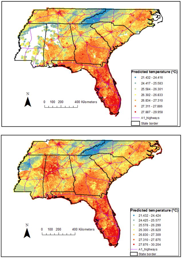
Predicted air temperature (°C) from stage 2 (top) and both stage 2 & 3 (bottom) in each 1 km × 1 km grid on a sample day (2011.08.25) across the southeastern USA.

The missing values of stage 2 can be filled using a stage 3 model, and the results are shown in Fig. 3 (bottom). The stage 3 model also performed well. The R² values between stage 3 and stage 2 predictions are shown in Appendix A (Table A.5), and the mean R² value for the entire study period is 0.971 (year-to-year variation 0.962 - 0.981). For the entire 15 years, 56.2% of the final predictions were derived from stage 3. There was still a small amount of missing predictions (1.4%) due to lack of monitored T_a measurements within 100 km buffer on a day. More details are in Table 2.

Table 2. Contribution of each stage for the daily T_a predictions for each year (2000-2014).

Year	Stage 2	Stage 3	Missing
2000	38.1%	60.4%	1.5%
2001	39.4%	59.2%	1.4%
2002	37.7%	60.9%	1.4%
2003	39.4%	59.1%	1.5%
2004	38.2%	60.6%	1.2%
2005	44.3%	54.6%	1.1%
2006	47.2%	51.7%	1.1%
2007	45.7%	53.2%	1.1%
2008	46.3%	52.6%	1.1%
2009	41.0%	57.9%	1.1%
2010	46.2%	52.2%	1.6%
2011	48.0%	50.0%	2.0%
2012	45.2%	52.9%	1.9%
2013	39.0%	59.7%	1.3%
2014	40.3%	58.6%	1.1%
Overall Mean	42.4%	56.2%	1.4%

Figure 4 illustrates the spatial pattern of estimated T_a values from the 3-stage statistical models, averaged over the year of 2011 for the southeastern USA area. In the calculation of the annual average, we removed grid cells with less than 243 observations (2/3 of the daily T_a predictions) in 2011. After restriction, estimated annual average T_a values across the study area for 2011 ranged from 10.91 °C to 25.91 °C. The figure shows that urban areas such as Raleigh, Atlanta, Birmingham, Jackson, Columbia, and Memphis, appear warmer than the surrounding areas possibly due to urban heat-island effect (25). In addition, estimated annual T_a values are higher in areas closer to the shoreline compared with inland areas as an impact of the ocean.

Fig. 4.

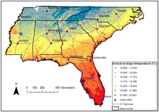
Spatial pattern of predicted air temperature (°C), averaged over the 2011 for the southeastern USA.

In addition to the spatial variability we observed, air temperature showed temporal variation in its spatial pattern as well. Figure 5 shows that there is space-time variation in the estimated T_a values for a subset of the study area. The results indicate that our model predictions can well resolve the day-to-day variation in the spatial pattern of T_a exposure.

Fig. 5.

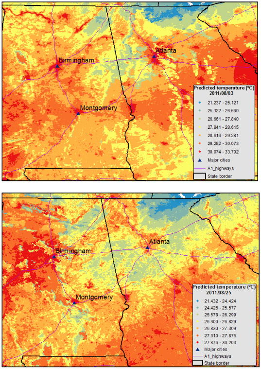
Predicted air temperature (°C) at a 1 km × 1 km grid for August 3, 2011 (top) and August 25, 2011 (bottom).

With respect to the final T_a exposure dataset that we generated, an independent validation was performed, by comparing our final daily T_a dataset with MERRA products T_2m. A good agreement was achieved, with an overall R² of 0.969 and RMSPE of 1.376 °C. The spatial and temporal R² values are 0.954 and 0.976, respectively. Results for the year 2011 are shown in Fig. 6 as an example. Comparison results for 15 years are compiled in Table 3.

Fig. 6.

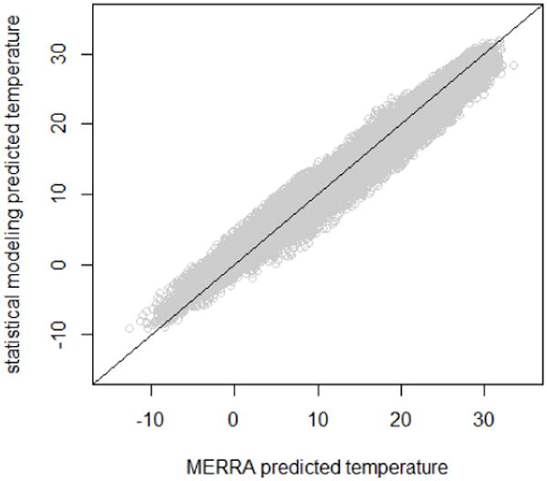
A scatter plot of the calculated daily average T_a versus the daily T_2m from MERRA. Data are shown for the year 2011.

Table 3. Prediction accuracy: R² for comparing final daily T_a predictions with MERRA products (2000-2014).

Year	CV R2	CV R2Spatial	CV R2Temporal	RMSPE	RMSPESpatial
2000	0.959	0.896	0.970	1.553	1.375
2001	0.964	0.955	0.972	1.388	1.095
2002	0.972	0.966	0.978	1.344	0.846
2003	0.974	0.958	0.981	1.245	0.876
2004	0.969	0.956	0.978	1.356	0.979
2005	0.971	0.955	0.979	1.328	0.871
2006	0.960	0.952	0.970	1.487	1.261
2007	0.965	0.951	0.971	1.456	1.154
2008	0.968	0.964	0.974	1.389	0.942
2009	0.971	0.965	0.981	1.342	0.970
2010	0.978	0.953	0.984	1.361	0.840
2011	0.969	0.964	0.976	1.423	0.969
2012	0.964	0.960	0.971	1.341	0.981
2013	0.972	0.965	0.980	1.288	0.960
2014	0.974	0.956	0.979	1.336	0.892
Overall Mean	0.969	0.954	0.976	1.376	1.001

4 Discussion

The southeastern USA is distinguished by its warm weather and serves as a place for relocation, particularly for the elderly who are most sensitive to climate change. The rapid population growth further urges epidemiological studies on the health effects of climate change in this area. Most temperature-related epidemiological studies have relied on central meteorological stations to assess T_a. The poor spatial resolution of monitor stations can result in exposure measurement error, with expected downward bias in estimating the health effects of temperature and elevated risk of not finding a significant association. This has been recently demonstrated in a study of temperature and birth weight in Massachusetts (27). As a result, recently increasing epidemiological studies have used the finer scale exposure estimates from remote sensing (28-30).

To the best of our knowledge, this work is the first study estimating spatially and temporally resolved air temperature for the southeastern USA with a humid subtropical climate. We presented several key features in our study. First, the T_a prediction models exhibited excellent model performances. We had no bias in the cross-validation results (average slope of 1.00). In contrast to the previous work by Kloog et al (2014) in the northeastern USA, we fit a more complex model for stage 3, which included important land use terms such as proximity to water, urbanization, and time varying covariates such as NDVI. Consequently, our stage 3 model had a higher R² (0.971) than was observed in the previous work (0.940). The results also compared well with reanalysis products, which were generated using an entirely different approach from statistical modeling.

Another key feature is that this study provides local temperature estimates on a daily basis within a study area for 15 years. Such a large 15-year daily exposure dataset will be particularly valuable for estimating the health effects of temperature in both short- and long-term, and locations outside of metropolitan areas, which are rarely included in epidemiology studies of temperature. In sum, our analysis showed that regardless of the quantity or quality of predictions, T_a can be reliably predicted from T_s if modeled appropriately.

Despite the high accuracy and low percent of missing of our model prediction, there are several limitations in the present study. For one the southeastern USA has many wetlands (swamps), which is part of the challenge of retrieving satellite T_s information. Even though 1 km is the finest resolution of T_s products that are available, Sabrino and coauthors reported that spatial resolutions lower than 50 m would underestimate the urban heat-island effect (31). In addition, this satellite-based approach still depends on ground T_a monitors. Without sufficient T_a monitors, the predictive power might be reduced dramatically, especially the mixed linear model. Because the mixed linear model uses a daily calibration method, thus requires relatively densely distributed daily T_a stations. In addition to ground T_a monitors, this satellite-based approach is also affected by some other factors, such as atmospheric conditions. Furthermore, daytime and nighttime temperatures detected by satellite are not daily mean temperatures. As a caveat, the T_a retrieved from this study should be considered as a high-resolution alternative for those areas with limited meteorological stations but cannot replace ground monitoring temperature.

In summary, we demonstrate how satellite-derived surface temperature can be used reliably to construct a high resolution dataset of daily air temperature. This dataset could well resolve and capture the spatial and temporal variations in T_a in warm areas. Public health burden of these variations should be investigated in future studies.

Highlights.

High resolution (1 km) daily air temperature was retrieved in Southeastern US.

Validations were conducted against weather stations and reanalysis.

High correlation and low bias were achieved.

Data are especially useful for public health studies.

References

- 1.Gosling SN, Lowe JA, McGregor GR, Pelling M, Malamud BD. Associations between elevated atmospheric temperature and human mortality: a critical review of the literature. Climatic Change. 2009;92(3-4):299–341. [Google Scholar]
- 2.Gosling SN, McGregor GR, Lowe JA. Climate change and heat-related mortality in six cities Part 2: climate model evaluation and projected impacts from changes in the mean and variability of temperature with climate change. International journal of biometeorology. 2009;53(1):31–51. doi: 10.1007/s00484-008-0189-9. [DOI] [PubMed] [Google Scholar]
- 3.Zanobetti A, Schwartz J. Temperature and mortality in nine US cities. Epidemiology (Cambridge, Mass) 2008;19(4):563–570. doi: 10.1097/EDE.0b013e31816d652d. [DOI] [PMC free article] [PubMed] [Google Scholar]
- 4.Medina-Ramón M, Schwartz J. Temperature, temperature extremes, and mortality: a study of acclimatisation and effect modification in 50 US cities. Occupational and environmental medicine. 2007;64(12):827–833. doi: 10.1136/oem.2007.033175. [DOI] [PMC free article] [PubMed] [Google Scholar]
- 5.Basu R. High ambient temperature and mortality: a review of epidemiologic studies from 2001 to 2008. Environ Health. 2009;8(1):40–52. doi: 10.1186/1476-069X-8-40. [DOI] [PMC free article] [PubMed] [Google Scholar]
- 6.Laaidi M, Laaidi K, Besancenot JP. Temperature-related mortality in France, a comparison between regions with different climates from the perspective of global warming. International journal of biometeorology. 2006;51(2):145–153. doi: 10.1007/s00484-006-0045-8. [DOI] [PubMed] [Google Scholar]
- 7.Xu Z, Etzel RA, Su H, Huang C, Guo Y, Tong S. Impact of ambient temperature on children's health: a systematic review. Environmental research. 2012;117:120–131. doi: 10.1016/j.envres.2012.07.002. [DOI] [PubMed] [Google Scholar]
- 8.Guo Y, Barnett AG, Tong S. Spatiotemporal model or time series model for assessing city-wide temperature effects on mortality? Environmental research. 2013;120:55–62. doi: 10.1016/j.envres.2012.09.001. [DOI] [PubMed] [Google Scholar]
- 9.Shi L, Kloog I, Zanobetti A, Liu P, Schwartz JD. Impacts of temperature and its variability on mortality in New England. Nature Climate Change. 2015 doi: 10.1038/nclimate2704. [DOI] [PMC free article] [PubMed] [Google Scholar]
- 10.Vicente Serrano SM, Sánchez S, Cuadrat JM. Comparative analysis of interpolation methods in the middle Ebro Valley (Spain): application to annual precipitation and temperature. Climate Research. 2003;24(2):161–180. [Google Scholar]
- 11.Hudson G, Wackernagel H. Mapping temperature using kriging with external drift: theory and an example from Scotland. International journal of Climatology. 1994;14(1):77–91. [Google Scholar]
- 12.Vancutsem C, Ceccato P, Dinku T, Connor SJ. Evaluation of MODIS land surface temperature data to estimate air temperature in different ecosystems over Africa. Remote Sensing of Environment. 2010;114(2):449–465. [Google Scholar]
- 13.Zhu W, Lű A, Jia S. Estimation of daily maximum and minimum air temperature using MODIS land surface temperature products. Remote Sensing of Environment. 2013;130:62–73. [Google Scholar]
- 14.Benali A, Carvalho A, Nunes J, Carvalhais N, Santos A. Estimating air surface temperature in Portugal using MODIS LST data. Remote Sensing of Environment. 2012;124:108–121. [Google Scholar]
- 15.Stoll MJ, Brazel AJ. Surface-air temperature relationships in the urban environment of Phoenix, Arizona. Physical Geography. 1992;13(2):160–179. [Google Scholar]
- 16.Voogt JA, Oke TR. Complete urban surface temperatures. Journal of Applied Meteorology. 1997;36(9):1117–1132. [Google Scholar]
- 17.Dousset B, editor. AVHRR-derived cloudiness and surface temperature patterns over the Los Angeles area and their relationships to land use; Geoscience and Remote Sensing Symposium, 1989 IGARSS'89 12th Canadian Symposium on Remote Sensing, 1989 International; 1989; IEEE; [Google Scholar]
- 18.Fu G, Shen Z, Zhang X, Shi P, Zhang Y, Wu J. Estimating air temperature of an alpine meadow on the Northern Tibetan Plateau using MODIS land surface temperature. Acta Ecologica Sinica. 2011;31(1):8–13. [Google Scholar]
- 19.Kloog I, Chudnovsky A, Koutrakis P, Schwartz J. Temporal and spatial assessments of minimum air temperature using satellite surface temperature measurements in Massachusetts, USA. Science of the Total Environment. 2012;432:85–92. doi: 10.1016/j.scitotenv.2012.05.095. [DOI] [PMC free article] [PubMed] [Google Scholar]
- 20.Kloog I, Nordio F, Coull BA, Schwartz J. Predicting spatiotemporal mean air temperature using MODIS satellite surface temperature measurements across the Northeastern USA. Remote Sensing of Environment. 2014;150:132–139. [Google Scholar]
- 21.Wan Z. New refinements and validation of the MODIS land-surface temperature/emissivity products. Remote Sensing of Environment. 2008;112(1):59–74. [Google Scholar]
- 22.Jin S, Yang L, Danielson P, Homer C, Fry J, Xian G. A comprehensive change detection method for updating the National Land Cover Database to circa 2011. Remote Sensing of Environment. 2013;132:159–175. [Google Scholar]
- 23.Maune DF. Digital elevation model technologies and applications: the DEM users manual. Asprs Publications; 2007. [Google Scholar]
- 24.Rienecker MM, Suarez MJ, Gelaro R, Todling R, Bacmeister J, Liu E, et al. MERRA: NASA's Modern-Era Retrospective Analysis for Research and Applications. Journal of climate. 2011;24(14):3624–3648. doi: 10.1175/JCLI-D-16-0758.1. [DOI] [PMC free article] [PubMed] [Google Scholar]
- 25.Kim HH. Urban heat island. International Journal of Remote Sensing. 1992;13(12):2319–2336. [Google Scholar]
- 26.Guo Y, Punnasiri K, Tong S, Aydin D, Feychting M. Effects of temperature on mortality in Chiang Mai city, Thailand: a time series study. Environ Health. 2012;11(36):10–1186. doi: 10.1186/1476-069X-11-36. [DOI] [PMC free article] [PubMed] [Google Scholar]
- 27.Kloog I, Melly SJ, Coull BA, Nordio F, Schwartz JD. Environmental health perspectives. 2015. Using Satellite-Based Spatiotemporal Resolved Air Temperature Exposure to Study the Association between Ambient Air Temperature and Birth Outcomes in Massachusetts. [DOI] [PMC free article] [PubMed] [Google Scholar]
- 28.Laaidi M, Zeghnoun A, Dousset B, Bretin P, Vandentorren S, Giraudet E, et al. The impact of heat islands on mortality in Paris during the August 2003 heat wave. Environmental Health Perspectives. 2012;120(2):254–259. doi: 10.1289/ehp.1103532. [DOI] [PMC free article] [PubMed] [Google Scholar]
- 29.Xu Z, Liu Y, Ma Z, Li S, Hu W, Tong S. Impact of temperature on childhood pneumonia estimated from satellite remote sensing. Environmental research. 2014;132:334–341. doi: 10.1016/j.envres.2014.04.021. [DOI] [PubMed] [Google Scholar]
- 30.Xu Z, Liu Y, Ma Z, Toloo GS, Hu W, Tong S. Assessment of the temperature effect on childhood diarrhea using satellite imagery. Scientific reports. 2014;4:5389. doi: 10.1038/srep05389. [DOI] [PMC free article] [PubMed] [Google Scholar]
- 31.Sobrino J, Oltra-Carrió R, Sòria G, Bianchi R, Paganini M. Impact of spatial resolution and satellite overpass time on evaluation of the surface urban heat island effects. Remote Sensing of Environment. 2012;117:50–56. [Google Scholar]
Associated Data
This section collects any data citations, data availability statements, or supplementary materials included in this article.